统计学习：logistic回归 Python实现

1. 最大熵模型

作用是从许多个模型中，选择一个最好的模型，选择的标准就是熵，即具有最大熵的$P(Y|X)$就是最好的模型。个人理解最大熵在这里起的作用类似于valid data 的作用。为什么最大熵的模型就是最好的呢？因为在自然界中，所有的分布都是趋于无序的、混乱的。最大熵准则则保留了每一种可能发生的情况，可以代表更多的可能发生的信息。比如你在猜抛掷一枚硬币，正面朝上的概率的时候，最好猜1/2而不是3/10.

2.Logistic回归

适用于多分类，二分类任务。注意：只适用于线性可分的任务，对于非线性的分类任务，logistic不能求解，此时可以适用svm等其它算法求解。分布函数是一个S形函数，记原始的训练集为 { ( x 1 , y 1 ) , ( x 2 , y 2 ) , ( x 3 , y 3 ) , . . . , ( x m , y m ) } \{(x_1,y_1), (x_2,y_2), (x_3,y_3), ..., (x_m,y_m) \} {(x1​,y1​),(x2​,y2​),(x3​,y3​),...,(xm​,ym​)}, $x_i\in {\mathbb{R}}^n$, y i ∈ { 1 , 2 , . . . , K } y_i\in \{1,2, ..., K\} yi​∈{1,2,...,K}。通过s函数，将$w^{T}x+b$ 的值域从$(-\infty ,+\infty )$映射为(0,1)。

3.代码实现

使用梯度下降法更新参数w,b

import numpy as np
import matplotlib.pyplot as plt


class LogisticClassifier:
    def __init__(self,learning_rate,epoch,delta):
        self.lr_rate = learning_rate
        self.epochs = epoch
        self.delta = delta
        self.w = None

    def sigmoid(self,x):
        return 1/(1+np.exp(-x))

    def fit(self,X_train,y_train):
        decent = 0
        y_train = y_train.T
        #print(y_train.shape)
        self.w = np.zeros(X_train.shape[1]).reshape(1,-1)  # 根据训练数据特征值的维数初始化参数w的维度以及形状
        for i in range(self.epochs):
            ## 计算W.T 点乘 x
            #print(i)        
            z = np.dot(X_train,self.w.T)  # M*N  (1*N).T
            h_theta = self.sigmoid(z)
            #print(h_theta.shape)
            error = h_theta - y_train  # y是一个列向量，计算误差 
            error_ = X_train*error
            # 计算梯度
            decent = error_.sum(axis=0)  ## 这个是梯度，并不是指的loss
                     
            if (np.abs(decent) <= self.delta).all():
                break
            else:
                self.w = self.w -self.lr_rate*decent
        print('Weight: ')
        print(self.w[0][:-1])
        print('bias:')
        print(self.w[0][-1])

    def predict(self,X_test):
        X_test = np.append(X_test,np.ones((X_test.shape[0],1)),axis=1)
        predic = self.sigmoid(np.dot(X_test,self.w.T))
        result = np.asarray((predic >= 0.5).astype(int))
        print('----------------------------')
        print('The predict label is :')
        print(result[0][0])

 if __name__ == '__main__':
    x1 = [3,3,3,1]
    x2 = [4,3,2,1]
    x3 = [2,1,2,1]
    x4 = [1,1,1,0]
    x5 = [-1,0,1,0]
    x6 = [2,-2,1,0]
    data = np.array([x1,x2,x3,x4,x5,x6]).reshape(6,-1)
    x_image = data[:,:-1] # 获得训练集中的特征值
    m,n = np.shape(x_image)                              # 获得feature的维度，m是样本个数，n是特征的维度
    x_image = np.append(x_image,np.ones((m,1)),axis = 1) # w.dot x + b 统一看作一个大的矩阵，用矩阵相乘表示这个运算过程。
    x_label = data[:,-1].reshape(1,-1)  # 获得训练集数据的标签值

    classifier = LogisticClassifier(learning_rate=0.1,epoch=100,delta=0.02)
    classifier.fit(x_image,x_label)
    X_test = np.array([1,2,-2]).reshape(1,-1)
    classifier.predict(X_test)

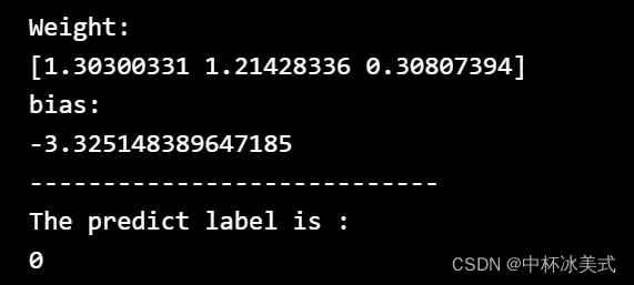
运行结果：