


1. KNN的介绍和应用
1.1 KNN的介绍
kNN(k-nearest neighbors),中文翻译K近邻。我们常常听到一个故事:如果要了解一个人的经济水平,只需要知道他最好的5个朋友的经济能力, 对他的这五个人的经济水平求平均就是这个人的经济水平。这句话里面就包含着kNN的算法思想。
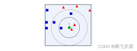
示例 :如上图,绿色圆要被决定赋予哪个类,是红色三角形还是蓝色四方形?如果K=3,由于红色三角形所占比例为2/3,绿色圆将被赋予红色三角形那个类,如果K=5,由于蓝色四方形比例为3/5,因此绿色圆被赋予蓝色四方形类。
1.1.1 KNN建立过程
- 给定测试样本,计算它与训练集中的每一个样本的距离。
- 找出距离近期的K个训练样本。作为测试样本的近邻。
- 依据这K个近邻归属的类别来确定样本的类别。
1.1.2 类别的判定
- 投票决定,少数服从多数。取类别最多的为测试样本类别。
- 加权投票法,依据计算得出距离的远近,对近邻的投票进行加权,距离越近则权重越大,设定权重为距离平方的倒数。
1.2 KNN的应用
KNN虽然很简单,但是人们常说"大道至简",一句"物以类聚,人以群分"就能揭开其面纱,看似简单的KNN即能做分类又能做回归, 还能用来做数据预处理的缺失值填充。由于KNN模型具有很好的解释性,一般情况下对于简单的机器学习问题,我们可以使用KNN作为 Baseline,对于每一个预测结果,我们可以很好的进行解释。推荐系统的中,也有着KNN的影子。例如文章推荐系统中, 对于一个用户A,我们可以把和A最相近的k个用户,浏览过的文章推送给A。
机器学习领域中,数据往往很重要,有句话叫做:“数据决定任务的上限, 模型的目标是无限接近这个上限”。 可以看到好的数据非常重要,但是由于各种原因,我们得到的数据是有缺失的,如果我们能够很好的填充这些缺失值, 就能够得到更好的数据,以至于训练出来更鲁棒的模型。接下来我们就来看看KNN如何做分类,怎么做回归以及怎么填充空值。
2. KNN 算法实战
2.1 Demo数据集
2.1.1 库函数导入
import numpy as np
import matplotlib.pyplot as plt
from matplotlib.colors import ListedColormap
from sklearn.neighbors import KNeighborsClassifier
from sklearn import datasets
2.1.2 数据导入
# 使用鸢尾花数据集的前两维数据,便于数据可视化
iris = datasets.load_iris()
X = iris.data[:,:2]
y = iris.target
2.1.3 模型训练&可视化
k_list = [1, 3, 5, 8, 10, 15]
h = .02
# 创建不同颜色的画布
cmap_light = ListedColormap(['orange', 'cyan', 'cornflowerblue'])
cmap_bold = ListedColormap(['darkorange', 'c', 'darkblue'])

plt.figure(figsize=(15,14))
# 根据不同的k值进行可视化
for ind,k in enumerate(k_list):
    clf = KNeighborsClassifier(k)
    clf.fit(X, y)
    # 画出决策边界
    x_min, x_max = X[:, 0].min() - 1, X[:, 0].max() + 1
    y_min, y_max = X[:, 1].min() - 1, X[:, 1].max() + 1
    xx, yy = np.meshgrid(np.arange(x_min, x_max, h),
                         np.arange(y_min, y_max, h))
    Z = clf.predict(np.c_[xx.ravel(), yy.ravel()])
    # 根据边界填充颜色
    Z = Z.reshape(xx.shape)

    plt.subplot(321+ind)
    plt.pcolormesh(xx, yy, Z, cmap=cmap_light)
    # 数据点可视化到画布
    plt.scatter(X[:, 0], X[:, 1], c=y, cmap=cmap_bold,
                edgecolor='k', s=20)
    plt.xlim(xx.min(), xx.max())
    plt.ylim(yy.min(), yy.max())
    plt.title("3-Class classification (k = %i)"% k)

plt.show()

2.1.4 原理简析
如果选择较小的K值,就相当于用较小的领域中的训练实例进行预测,例如当k=1的时候,在分界点位置的数据很容易受到局部的影响,图中蓝色的部分中还有部分绿色块,主要是数据太局部敏感。当k=15的时候,不同的数据基本根据颜色分开,当时进行预测的时候,会直接落到对应的区域,模型相对更加鲁棒。
2.2 鸢尾花数据集
2.2.1 库函数导入
import numpy as np
# 加载鸢尾花数据集
from sklearn import datasets
# 导入KNN分析器
from sklearn.neighbors import KNeighborsClassifier
from sklearn.model_selection import train_test_split
2.2.2 数据导入&分析
# 导入鸢尾花数据集
iris = datasets.load_iris()
X = iris.data
y = iris.target

# 得到训练集合和验证集合,8:2
X_train, X_test, y_train, y_test = train_test_split(X, y, test_size=0.2)
2.2.3 模型训练
这里我们设置参数k(n_neighbors)=5, 使用欧式距离(metric=minkowski & p=2)
# 训练模型
clf = KNeighborsClassifier(n_neighbors=5, p=2, metric="minkowski")
clf.fit(X_train, y_train)
KNeighborsClassifier()In a Jupyter environment, please rerun this cell to show the HTML representation or trust the notebook.
On GitHub, the HTML representation is unable to render, please try loading this page with nbviewer.org.
KNeighborsClassifier()
2.2.4 模型预测&可视化
# 预测
X_pred = clf.predict(X_test)
acc = sum(X_pred == y_test) / X_pred.shape[0]
print("预测的准确率 ACC:%.3f" % acc)
# 得分
print(clf.score(X_test, y_test))
预测的准确率 ACC:0.967
0.9666666666666667
我们用表格来看一下KNN的训练和预测过程。这里用表格进行可视化:
- 训练数据[表格对应list]
- knn.fit(X, y)的过程可以简单认为是表格存储
- knn.predict(x)预测过程会计算x和所有训练数据的距离 这里我们使用欧式距离进行计算, 预测过程如下
x
=
[
5.
,
3.6
,
1.4
,
0.2
]
x=[5.,3.6,1.4,0.2]
x=[5.,3.6,1.4,0.2]
y
=
0
y=0
y=0
step1: 计算x和所有训练数据的距离
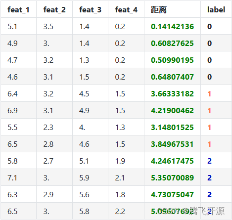
step2: 根据距离进行编号排序
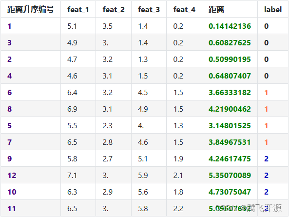
step3: 我们设置k=5,选择距离最近的k个样本进行投票
step4: k近邻的label进行投票
nn_labels = [0, 0, 0, 0, 1] --> 得到最后的结果0。
2.3 模拟数据集
2.3.1 库函数导入
#Demo来自sklearn官网
import numpy as np
import matplotlib.pyplot as plt
from sklearn.neighbors import KNeighborsRegressor
2.3.2 数据导入&分析
# 先定义一个随机数种子
np.random.seed(0)
# 随机生成40个(0, 1)之前的数,乘以5,再进行升序
X = np.sort(5 * np.random.rand(40, 1), axis=0)
# 创建[0, 5]之间的500个数的等差数列, 作为测试数据
T = np.linspace(0, 5, 500)[:, np.newaxis]
# 使用sin函数得到y值,并拉伸到一维
y = np.sin(X).ravel()
# Add noise to targets[y值增加噪声]
y[::5] += 1 * (0.5 - np.random.rand(8))
2.3.3 模型训练&预测可视化
# Fit regression model
# 设置多个k近邻进行比较
n_neighbors = [1, 3, 5, 8, 10, 40]
# 设置图片大小
plt.figure(figsize=(10,20))
for i, k in enumerate(n_neighbors):
    # 默认使用加权平均进行计算predictor
    clf = KNeighborsRegressor(n_neighbors=k, p=2, metric="minkowski")
    # 训练
    clf.fit(X, y)
    # 预测
    y_ = clf.predict(T)
    plt.subplot(6, 1, i + 1)
    plt.scatter(X, y, color='red', label='data')
    plt.plot(T, y_, color='navy', label='prediction')
    plt.axis('tight')
    plt.legend()
    plt.title("KNeighborsRegressor (k = %i)" % (k))

plt.tight_layout()
plt.show()

2.3.4 模型分析
当k=1时,预测的结果只和最近的一个训练样本相关,从预测曲线中可以看出当k很小时候很容易发生过拟合。
当k=40时,预测的结果和最近的40个样本相关,因为我们只有40个样本,此时是所有样本的平均值,此时所有预测值都是均值,很容易发生欠拟合。
一般情况下,使用knn的时候,根据数据规模我们会从[3, 20]之间进行尝试,选择最好的k,例如上图中的[3, 10]相对1和40都是还不错的选择。
2.4 马绞痛数据
2.4.1 库函数导入
import numpy as np
import pandas as pd
# KNN分类器
from sklearn.neighbors import KNeighborsClassifier
# KNN数据空值填充
from sklearn.impute import KNNImputer
# 计算带有空值的欧式距离
from sklearn.metrics.pairwise import nan_euclidean_distances
# 交叉验证
from sklearn.model_selection import cross_val_score
# KFlod的函数
from sklearn.model_selection import RepeatedStratifiedKFold
from sklearn.pipeline import Pipeline
import matplotlib.pyplot as plt
from sklearn.model_selection import train_test_split
2.4.2 数据导入&分析
数据中的’?‘表示空值,如果我们使用KNN分类器,’?'不是数值,不能进行计算,因此我们需要进行数据预处理对空值进行填充。
data = pd.read_csv("./data/horse-colic.csv")
data.head()
| 2 | 1 | 530101 | 38.50 | 66 | 28 | 3 | 3.1 | ? | 2.1 | ... | 45.00 | 8.40 | ?.4 | ?.5 | 2.2 | 2.3 | 11300 | 00000 | 00000.1 | 2.4 | |
|---|---|---|---|---|---|---|---|---|---|---|---|---|---|---|---|---|---|---|---|---|---|
| 0 | 1 | 1 | 534817 | 39.2 | 88 | 20 | ? | ? | 4 | 1 | ... | 50 | 85 | 2 | 2 | 3 | 2 | 2208 | 0 | 0 | 2 |
| 1 | 2 | 1 | 530334 | 38.30 | 40 | 24 | 1 | 1 | 3 | 1 | ... | 33.00 | 6.70 | ? | ? | 1 | 2 | 0 | 0 | 0 | 1 |
| 2 | 1 | 9 | 5290409 | 39.10 | 164 | 84 | 4 | 1 | 6 | 2 | ... | 48.00 | 7.20 | 3 | 5.30 | 2 | 1 | 2208 | 0 | 0 | 1 |
| 3 | 2 | 1 | 530255 | 37.30 | 104 | 35 | ? | ? | 6 | 2 | ... | 74.00 | 7.40 | ? | ? | 2 | 2 | 4300 | 0 | 0 | 2 |
| 4 | 2 | 1 | 528355 | ? | ? | ? | 2 | 1 | 3 | 1 | ... | ? | ? | ? | ? | 1 | 2 | 0 | 0 | 0 | 2 |
5 rows × 28 columns
这里我们使用KNNImputer进行空值填充,KNNImputer填充的原理很简单,计算每个样本最近的k个样本,进行空值填充。
我们先来看下KNNImputer的运行原理。
2.4.3 KNNImputer空值填充–使用和原理介绍
X = [[1, 2, np.nan], [3, 4, 3], [np.nan, 6, 5], [8, 8, 7]]
imputer = KNNImputer(n_neighbors=2, metric='nan_euclidean')
imputer.fit_transform(X)
array([[1. , 2. , 4. ],
       [3. , 4. , 3. ],
       [5.5, 6. , 5. ],
       [8. , 8. , 7. ]])
带有空值的欧式距离计算公式
nan_euclidean_distances([[np.nan, 6, 5], [3, 4, 3]], [[3, 4, 3], [1, 2, np.nan], [8, 8, 7]])
array([[3.46410162, 6.92820323, 3.46410162],
       [0.        , 3.46410162, 7.54983444]])
2.4.4 KNNImputer空值填充–欧式距离的计算
样本[1, 2, np.nan] 最近的2个样本是: [3, 4, 3] [np.nan, 6, 5], 计算距离的时候使用欧式距离,只关注非空样本。 [1, 2, np.nan] 填充之后得到 [1, 2, (3 + 5) / 2] = [1, 2, 4]
正常的欧式距离
x = [ 3 , 4 , 3 ] , y = [ 8 , 8 , 7 ] x=[3,4,3],y=[8,8,7] x=[3,4,3],y=[8,8,7]
( 3 − 8 ) 2 + ( 4 − 8 ) 2 + ( 3 − 7 ) 2 = 33 = 7.55 \sqrt{(3-8)^2+(4-8)^2+(3-7)^2}=\sqrt{33}=7.55 (3−8)2+(4−8)2+(3−7)2=33=7.55
带有空值的欧式聚类
x = [ 1 , 2 , n p . n a n ] , y = [ n p . n a n , 6 , 5 ] x=[1,2,np.nan],y=[np.nan,6,5] x=[1,2,np.nan],y=[np.nan,6,5]
3 1 ( 2 − 6 ) 2 = 48 = 6.928 \sqrt{\frac{3}{1}(2-6)^2}=\sqrt{48}=6.928 13(2−6)2=48=6.928
只计算所有非空的值,对所有空加权到非空值的计算上,上例中,我们看到一个有3维,只有第二维全部非空, 将第一维和第三维的计算加到第二维上,所有需要乘以3。
表格中距离度量使用的是带有空值欧式距离计算相似度,使用简单的加权平均进行填充。

# load dataset, 将?变成空值
input_file = './data/horse-colic.csv'
df_data = pd.read_csv(input_file, header=None, na_values='?')
df_data.head()
| 0 | 1 | 2 | 3 | 4 | 5 | 6 | 7 | 8 | 9 | ... | 18 | 19 | 20 | 21 | 22 | 23 | 24 | 25 | 26 | 27 | |
|---|---|---|---|---|---|---|---|---|---|---|---|---|---|---|---|---|---|---|---|---|---|
| 0 | 2.0 | 1 | 530101 | 38.5 | 66.0 | 28.0 | 3.0 | 3.0 | NaN | 2.0 | ... | 45.0 | 8.4 | NaN | NaN | 2.0 | 2 | 11300 | 0 | 0 | 2 |
| 1 | 1.0 | 1 | 534817 | 39.2 | 88.0 | 20.0 | NaN | NaN | 4.0 | 1.0 | ... | 50.0 | 85.0 | 2.0 | 2.0 | 3.0 | 2 | 2208 | 0 | 0 | 2 |
| 2 | 2.0 | 1 | 530334 | 38.3 | 40.0 | 24.0 | 1.0 | 1.0 | 3.0 | 1.0 | ... | 33.0 | 6.7 | NaN | NaN | 1.0 | 2 | 0 | 0 | 0 | 1 |
| 3 | 1.0 | 9 | 5290409 | 39.1 | 164.0 | 84.0 | 4.0 | 1.0 | 6.0 | 2.0 | ... | 48.0 | 7.2 | 3.0 | 5.3 | 2.0 | 1 | 2208 | 0 | 0 | 1 |
| 4 | 2.0 | 1 | 530255 | 37.3 | 104.0 | 35.0 | NaN | NaN | 6.0 | 2.0 | ... | 74.0 | 7.4 | NaN | NaN | 2.0 | 2 | 4300 | 0 | 0 | 2 |
5 rows × 28 columns
# 得到训练数据和label, 第23列表示是否发生病变, 1: 表示Yes; 2: 表示No.
data = df_data.values
ix = [i for i in range(data.shape[1]) if i != 23]
X, y = data[:, ix], data[:, 23]
# 查看所有特征的缺失值个数和缺失率
for i in range(df_data.shape[1]):
    n_miss = df_data[[i]].isnull().sum()
    perc = n_miss / df_data.shape[0] * 100
    if n_miss.values[0] > 0:
        print('>Feat: %d, Missing: %d, Missing ratio: (%.2f%%)' % (i, n_miss, perc))

# 查看总的空值个数
print('KNNImputer before Missing: %d' % sum(np.isnan(X).flatten()))
>Feat: 0, Missing: 1, Missing ratio: (0.33%)
>Feat: 3, Missing: 60, Missing ratio: (20.00%)
>Feat: 4, Missing: 24, Missing ratio: (8.00%)
>Feat: 5, Missing: 58, Missing ratio: (19.33%)
>Feat: 6, Missing: 56, Missing ratio: (18.67%)
>Feat: 7, Missing: 69, Missing ratio: (23.00%)
>Feat: 8, Missing: 47, Missing ratio: (15.67%)
>Feat: 9, Missing: 32, Missing ratio: (10.67%)
>Feat: 10, Missing: 55, Missing ratio: (18.33%)
>Feat: 11, Missing: 44, Missing ratio: (14.67%)
>Feat: 12, Missing: 56, Missing ratio: (18.67%)
>Feat: 13, Missing: 104, Missing ratio: (34.67%)
>Feat: 14, Missing: 106, Missing ratio: (35.33%)
>Feat: 15, Missing: 247, Missing ratio: (82.33%)
>Feat: 16, Missing: 102, Missing ratio: (34.00%)
>Feat: 17, Missing: 118, Missing ratio: (39.33%)
>Feat: 18, Missing: 29, Missing ratio: (9.67%)
>Feat: 19, Missing: 33, Missing ratio: (11.00%)
>Feat: 20, Missing: 165, Missing ratio: (55.00%)
>Feat: 21, Missing: 198, Missing ratio: (66.00%)
>Feat: 22, Missing: 1, Missing ratio: (0.33%)
KNNImputer before Missing: 1605


C:\Users\49269\AppData\Local\Temp\ipykernel_8948\2430280379.py:6: FutureWarning: Calling int on a single element Series is deprecated and will raise a TypeError in the future. Use int(ser.iloc[0]) instead
  print('>Feat: %d, Missing: %d, Missing ratio: (%.2f%%)' % (i, n_miss, perc))
C:\Users\49269\AppData\Local\Temp\ipykernel_8948\2430280379.py:6: FutureWarning: Calling float on a single element Series is deprecated and will raise a TypeError in the future. Use float(ser.iloc[0]) instead
  print('>Feat: %d, Missing: %d, Missing ratio: (%.2f%%)' % (i, n_miss, perc))
# 定义 knnimputer
imputer = KNNImputer()
# 填充数据集中的空值
imputer.fit(X)
# 转换数据集
Xtrans = imputer.transform(X)
# 打印转化后的数据集的空值
print('KNNImputer after Missing: %d' % sum(np.isnan(Xtrans).flatten()))
KNNImputer after Missing: 0
2.4.5 基于pipeline模型训练&可视化
什么是Pipeline, 我这里直接翻译成数据管道。任何有序的操作都可以看做pipeline,例如工厂流水线,对于机器学习模型来说,这就是数据流水线。 是指数据通过管道中的每一个节点,结果除了之后,继续流向下游。对于我们这个例子,数据是有空值,我们会有一个KNNImputer节点用来填充空值, 之后继续流向下一个kNN分类节点,最后输出模型。

results = list()
strategies = [str(i) for i in [1, 2, 3, 4, 5, 6, 7, 8, 9, 10, 15, 16, 18, 20, 21]]
for s in strategies:
    # create the modeling pipeline
    pipe = Pipeline(steps=[('imputer', KNNImputer(n_neighbors=int(s))), ('model', KNeighborsClassifier())])
    # 数据多次随机划分取平均得分
    scores = []
    for k in range(20):
        # 得到训练集合和验证集合, 8: 2
        X_train, X_test, y_train, y_test = train_test_split(Xtrans, y, test_size=0.2)
        pipe.fit(X_train, y_train)
        # 验证model
        score = pipe.score(X_test, y_test)
        scores.append(score)
    # 保存results
    results.append(np.array(scores))
    print('>k: %s, Acc Mean: %.3f, Std: %.3f' % (s, np.mean(scores), np.std(scores)))
# print(results)
# plot model performance for comparison
plt.boxplot(results, labels=strategies, showmeans=True)
plt.show()
>k: 1, Acc Mean: 0.812, Std: 0.041
>k: 2, Acc Mean: 0.832, Std: 0.051
>k: 3, Acc Mean: 0.826, Std: 0.046
>k: 4, Acc Mean: 0.813, Std: 0.046
>k: 5, Acc Mean: 0.814, Std: 0.043
>k: 6, Acc Mean: 0.805, Std: 0.052
>k: 7, Acc Mean: 0.826, Std: 0.033
>k: 8, Acc Mean: 0.838, Std: 0.041
>k: 9, Acc Mean: 0.812, Std: 0.029
>k: 10, Acc Mean: 0.818, Std: 0.050
>k: 15, Acc Mean: 0.802, Std: 0.039
>k: 16, Acc Mean: 0.814, Std: 0.047
>k: 18, Acc Mean: 0.824, Std: 0.041
>k: 20, Acc Mean: 0.810, Std: 0.047
>k: 21, Acc Mean: 0.812, Std: 0.044

2.4.6 结果分析
我们的实验是每个k值下,随机切分20次数据, 从上述的图片中, 根据k值的增加,我们的测试准确率会有先上升再下降再上升的过程。 [3, 5]之间是一个很好的取值,上文我们提到,k很小的时候会发生过拟合,k很大时候会发生欠拟合,当遇到第一下降节点,此时我们可以简单认为不再发生过拟合,取当前的k值即可。
2.5 KNN原理介绍
k近邻方法是一种惰性学习算法,可以用于回归和分类,它的主要思想是投票机制,对于一个测试实例x, 我们在有标签的训练数据集上找到和最相近的k个数据,用他们的label进行投票,分类问题则进行表决投票,回归问题使用加权平均或者直接平均的方法。knn算法中我们最需要关注两个问题:k值的选择和距离的计算。 kNN中的k是一个超参数,需要我们进行指定,一般情况下这个k和数据有很大关系,都是交叉验证进行选择,但是建议使用交叉验证的时候,k∈[2,20],使用交叉验证得到一个很好的k值。
k值还可以表示我们的模型复杂度,当k值越小意味着模型复杂度变大,更容易过拟合,(用极少数的样例来绝对这个预测的结果,很容易产生偏见,这就是过拟合)。我们有这样一句话,k值越多学习的估计误差越小,但是学习的近似误差就会增大。
距离/相似度的计算:
样本之间的距离的计算,我们一般使用Lp距离进行计算。当p=1时候,称为曼哈顿距离(Manhattan distance),当p=2时候,称为欧氏距离(Euclidean distance),当p=∞时候,称为极大距离(infty distance), 表示各个坐标的距离最大值,另外也包含夹角余弦等方法。
一般采用欧式距离较多,但是文本分类则倾向于使用余弦来计算相似度。
对于两个向量 ( x i , x j ) (x_i,x_j) (xi,xj) ,一般使用 L p L_p Lp 距离进行计算。假设特征空间 X 是 n 维实数向量空间 R n R^n Rn,其中, x i , x j ∈ X , x i = ( x i ( 1 ) , x i ( 2 ) , . . . , x i ( n ) ) , x j = ( x j ( 1 ) , x j ( 2 ) , . . . , x j ( n ) ) x i , x i , x j 的 L p x_i,x_j \in X, x_i=(x_i^{(1)},x_i^{(2)},...,x_i^{(n)}),x_j=(x_j^{(1)},x_j^{(2)},...,x_j^{(n)})x_i,x_i, x_j 的 L_p xi,xj∈X,xi=(xi(1),xi(2),...,xi(n)),xj=(xj(1),xj(2),...,xj(n))xi,xi,xj的Lp 距离定义为:
L p ( x i , x j ) = ( ∑ i = 1 n ∣ x j ( l ) − x j ( l ) ∣ p ) 1 p L_p(x_i,x_j)=(\sum_{i=1}^{n}|x_j^{(l)}-x_j^{(l)}|^{p})^{\frac{1}{p}} Lp(xi,xj)=(∑i=1n∣xj(l)−xj(l)∣p)p1
这里的 p ≥ 1 p \ge 1 p≥1。当 p = 2 时,成为欧氏距离(Euclidean distance):
L 2 ( x i , x j ) = ( ∑ l = 1 n ∣ x i ( l ) − x j ( l ) ∣ 2 ) 1 2 L_2(x_i,x_j)=(\sum_{l=1}^{n}|x_i^{(l)}-x_j^{(l)}|^{2})^{\frac{1}{2}} L2(xi,xj)=(∑l=1n∣xi(l)−xj(l)∣2)21
当 p = 1 时,成为曼哈顿距离(Manhattan distance):
L 1 ( X i , x j ) = ∑ l = 1 n ∣ x i ( l ) − x j ( l ) ∣ L_1(X_i,x_j)=\sum_{l=1}^{n}|x_i^{(l)}-x_j^{(l)}| L1(Xi,xj)=∑l=1n∣xi(l)−xj(l)∣
当 p = ∞ p = \infty p=∞ 时,成为极大距离(infty distance),表示各个坐标的距离最大值:
L p ( x i , x j ) = max l n ∣ x i ( l ) − x j ( l ) ∣ L_p(x_i,x_j)=\max_{l}n|x_i^{(l)}-x_j^{(l)}| Lp(xi,xj)=maxln∣xi(l)−xj(l)∣


 761
761

 被折叠的 条评论
为什么被折叠?
被折叠的 条评论
为什么被折叠?
 到【灌水乐园】发言


