Machine Learning Week 3

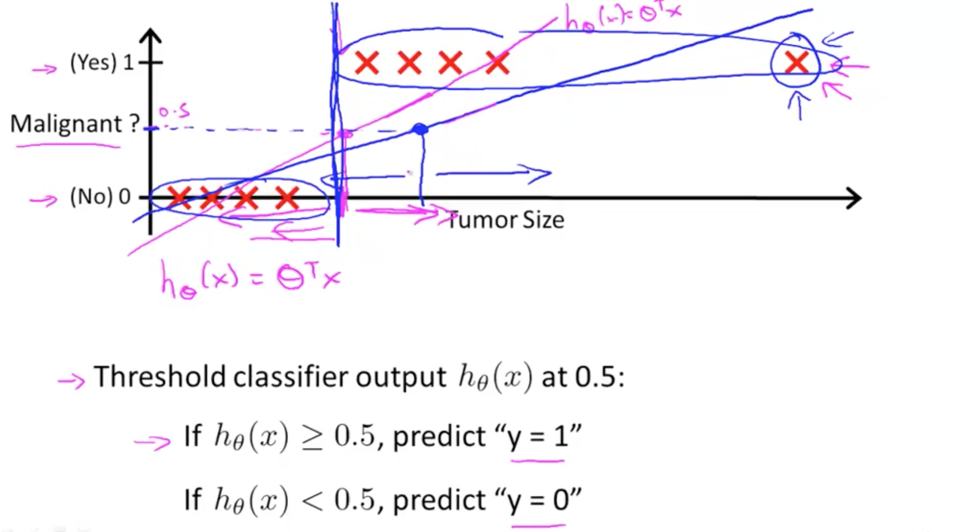
Linear Regression can’t be used for Classification Problems

Linear Regression isn’t Working Well for Regression Problem

An extra unusual point may affect all the linear function thus cause some error in the classification process.

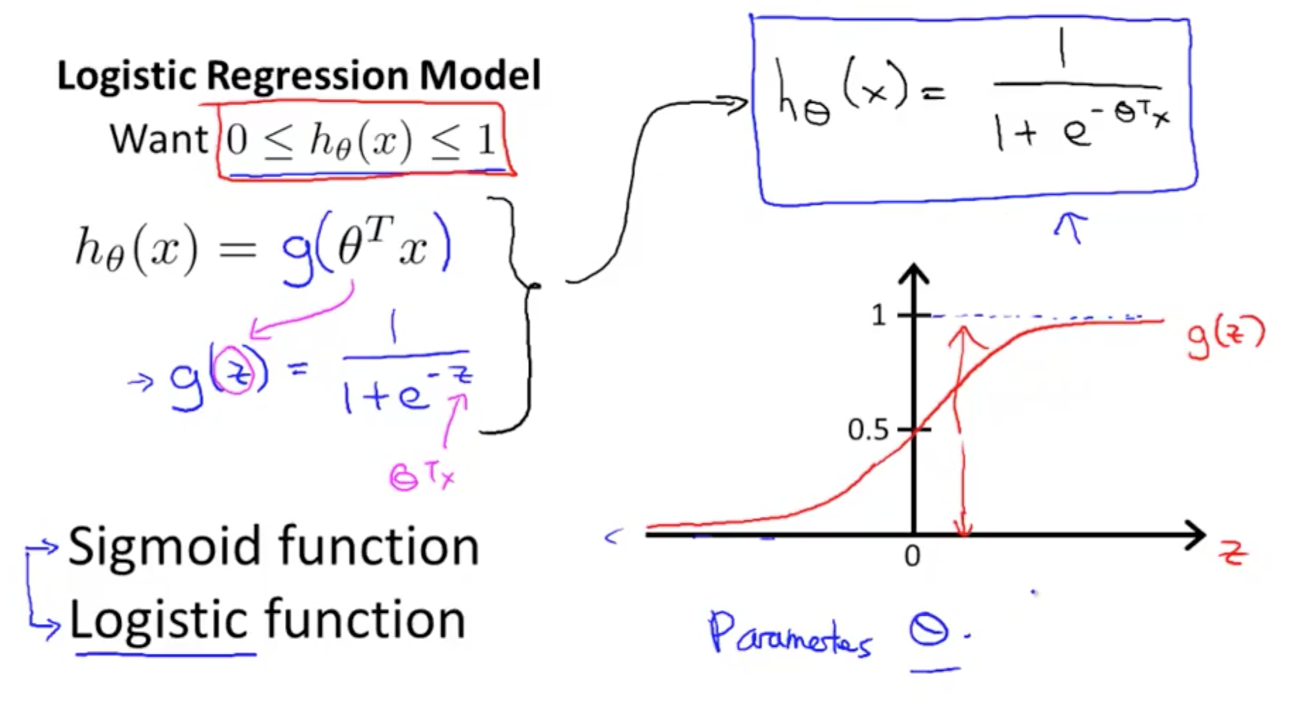
Logistic Regression Model

Sigmoid Function or Logistic Function

$$h_\theta(x)=g(\theta^Tx)$$
$$g(Z)=\frac{1}{1+e^{-Z}}$$

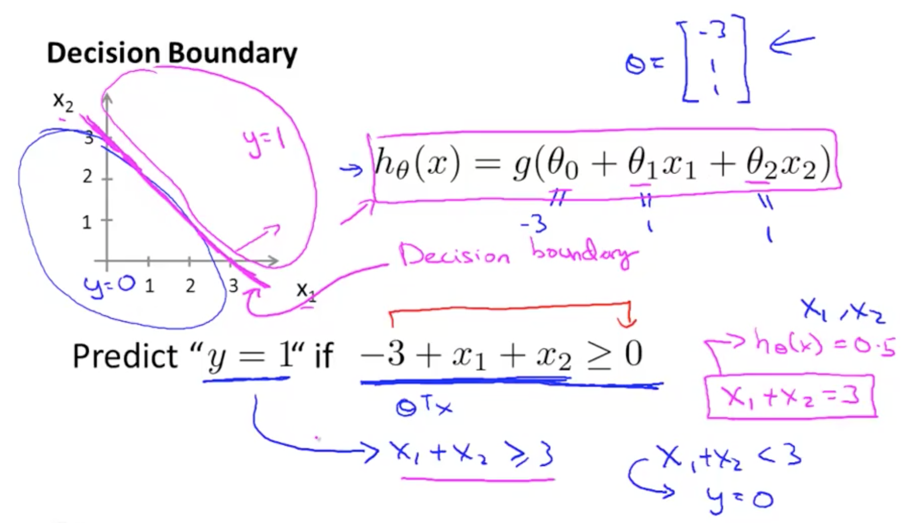
Decision Boundary

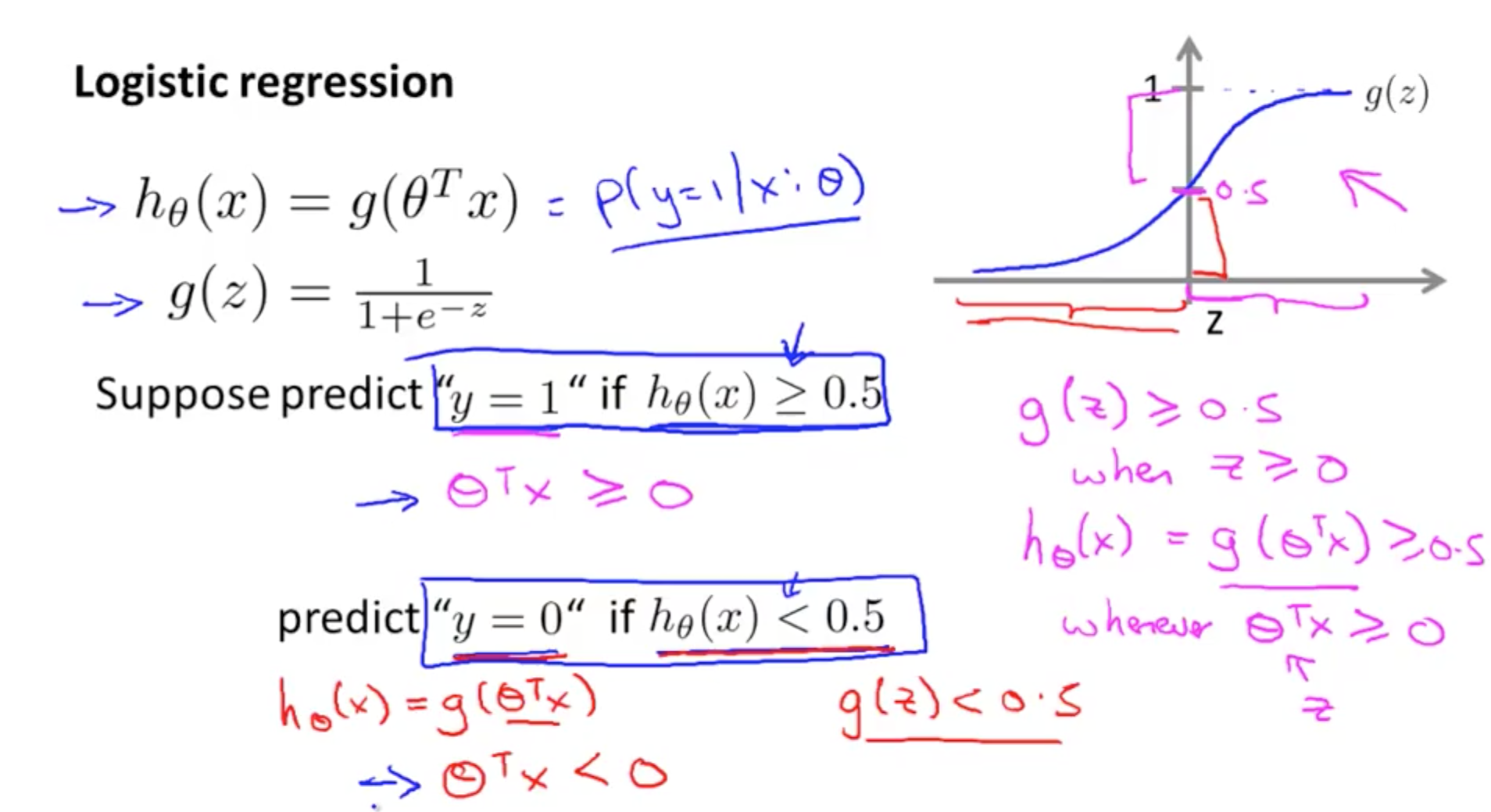
The predict is that if $h_\theta(x)\ge0.5$,then $y=1$,and if $h_\theta(x)\lt0.5$,then $y=0$ which is also equivalent to that if $\theta^Tx\ge0$,then $y=1$ and if $\theta^Tx\lt0$,then $y=0$

Example:

Cost Function and Gradient Descent for Logistic Regression

Cost Function for Logistic Regression

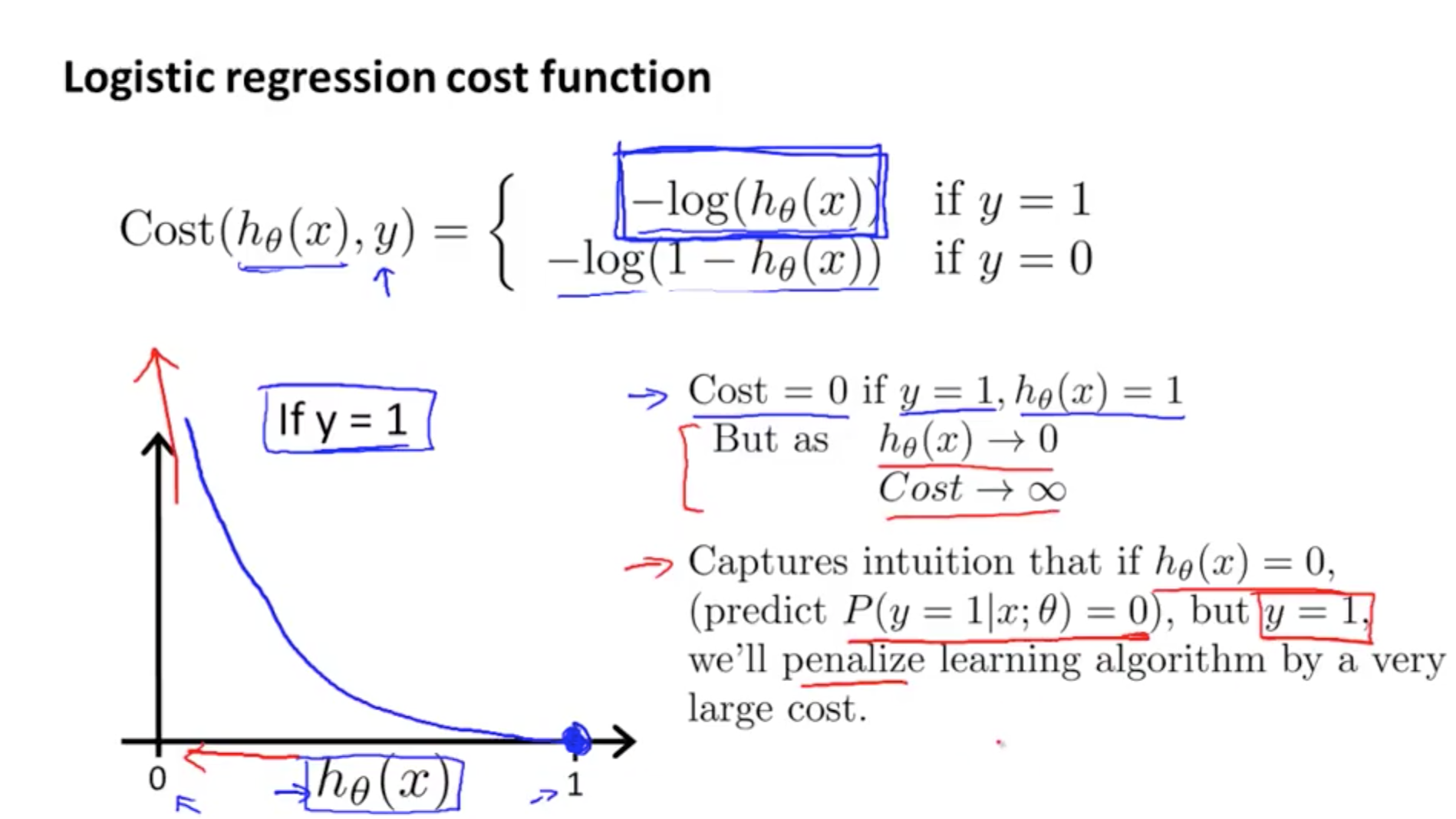
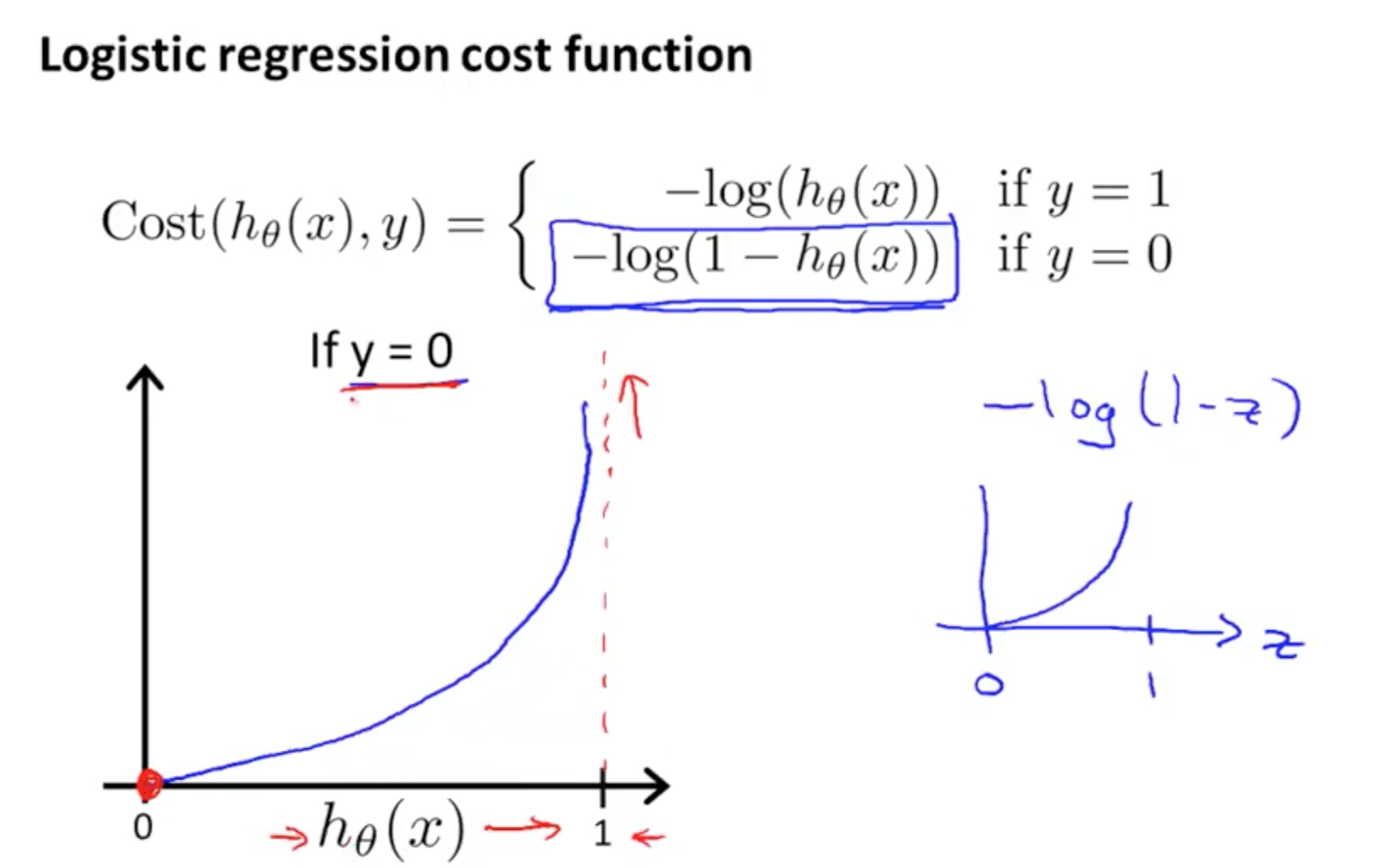
Together will be:

$$J(\theta)=\frac{1}{m}\sum_{i=1}^mCost(h_\theta(x^{(i)}),y^{(i)})$$

for linear regression:

$$Cost(h_\theta(x^{(i)}),y^{(i)})=\frac12(h_\theta(x{(i)})-y{(i)})^2$$

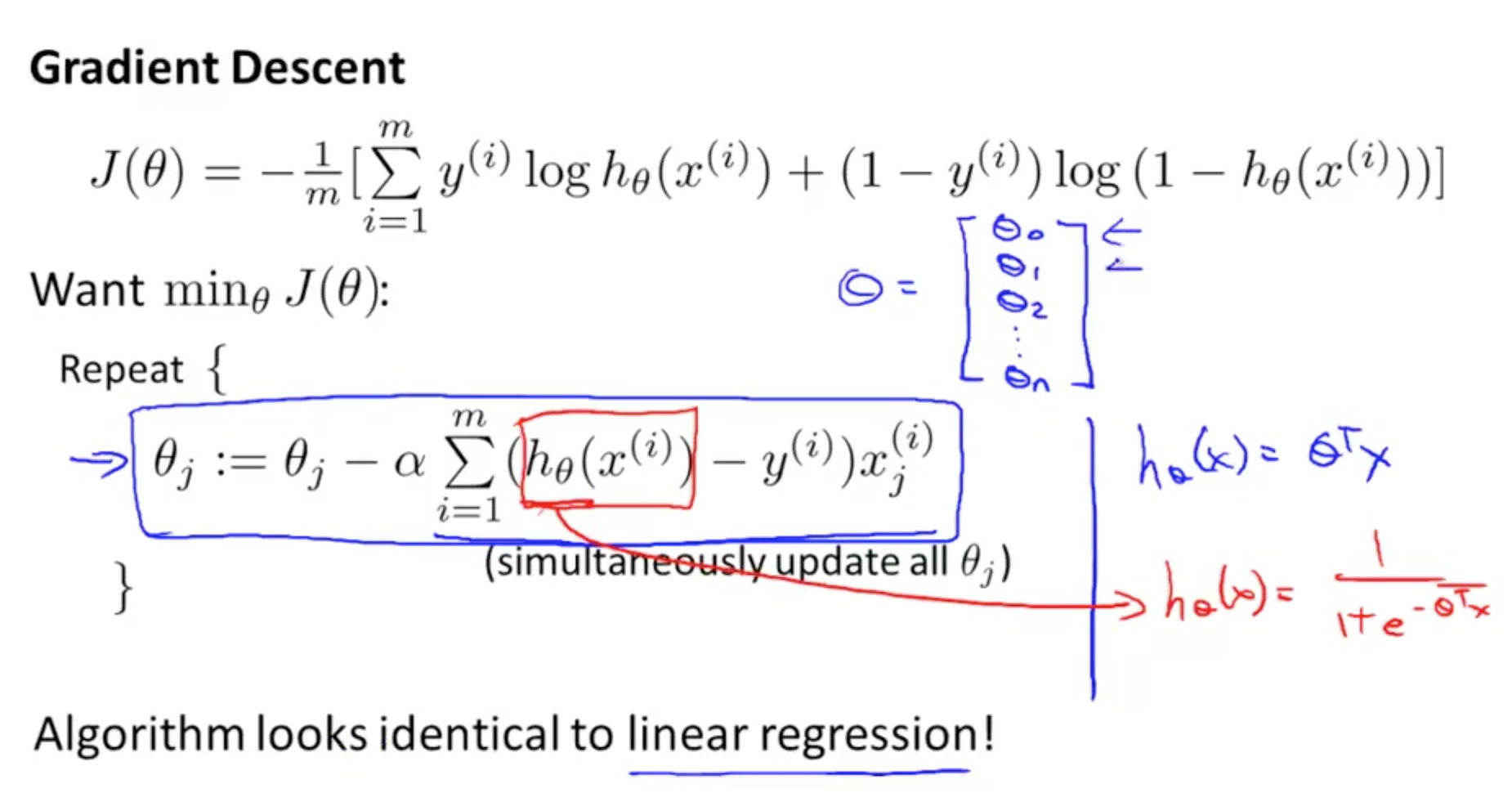
for logistic regression:

$$Cost(h_\theta(x),y)=-ylog(h_\theta(x)-(1-y)log(1-h_\theta(x))$$

Gradient descent of logistic regression is the same with linear regression

$$\theta_j:=\theta_j-\alpha\sum^m_{i=1}(h_\theta(x^{(i)})-y^{(i)})x_j^{(i)}$$

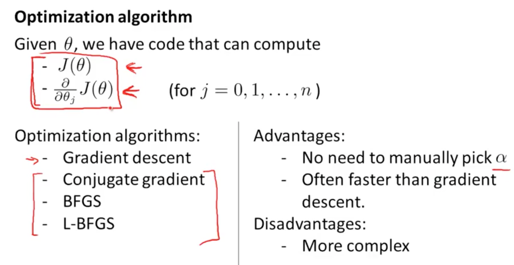
Several different way of optimization algorithm

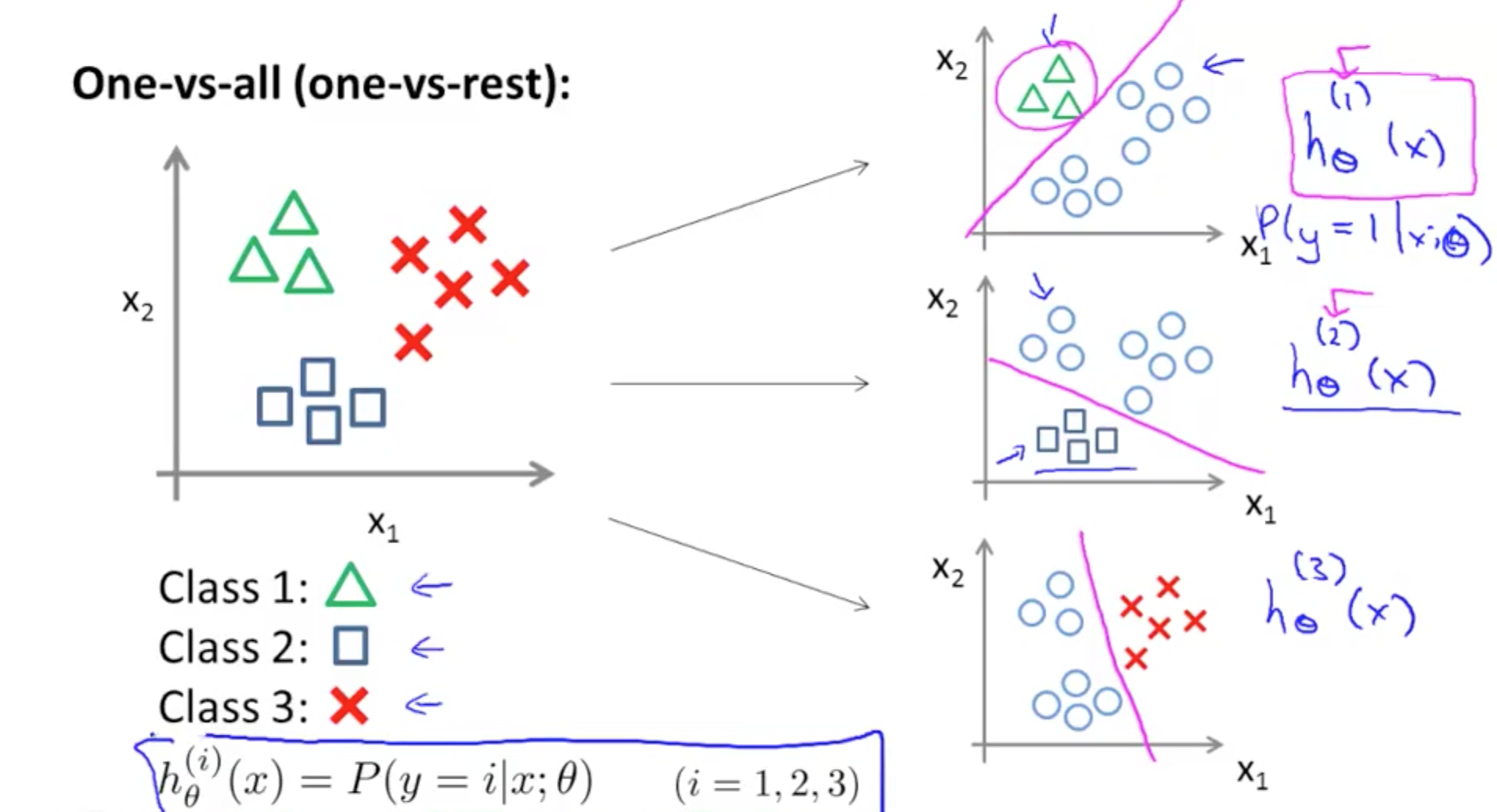
Multiclass Classification

One Vs All

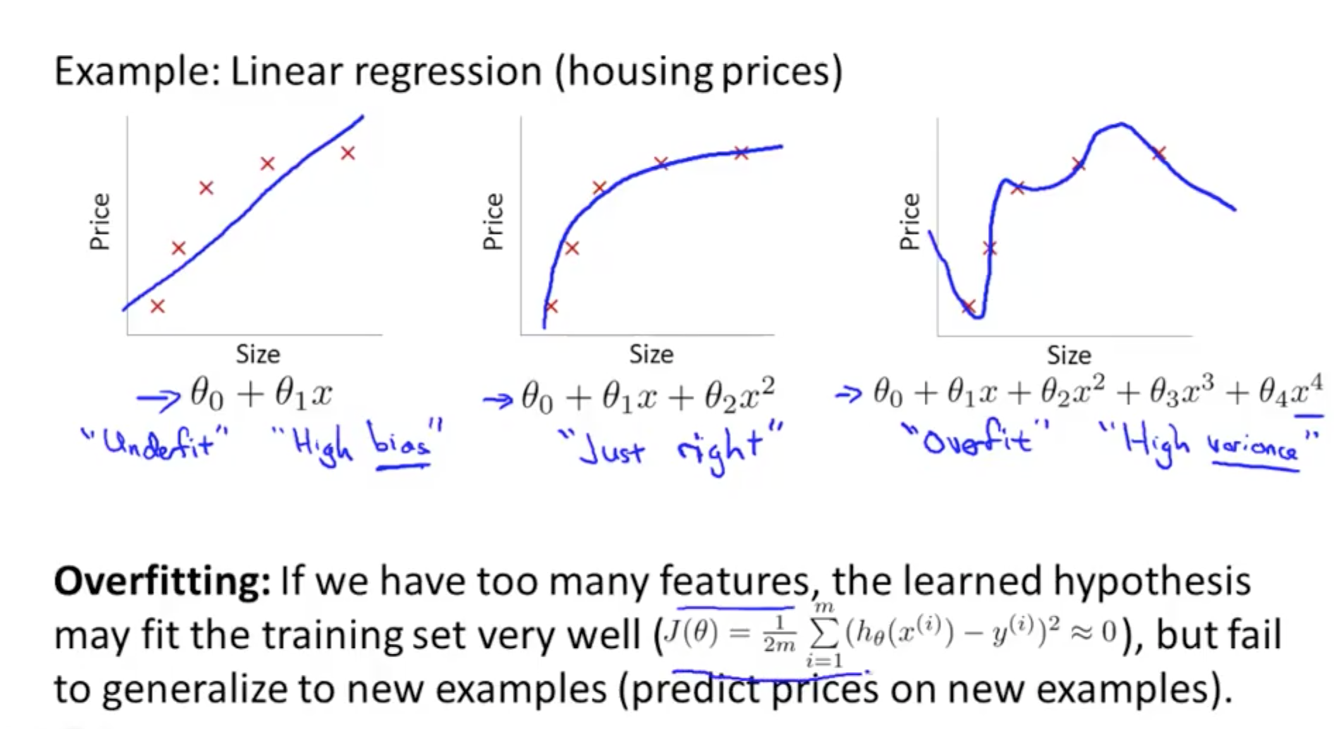
Problem of Overfitting

Under fitting - Just right - Over fitting

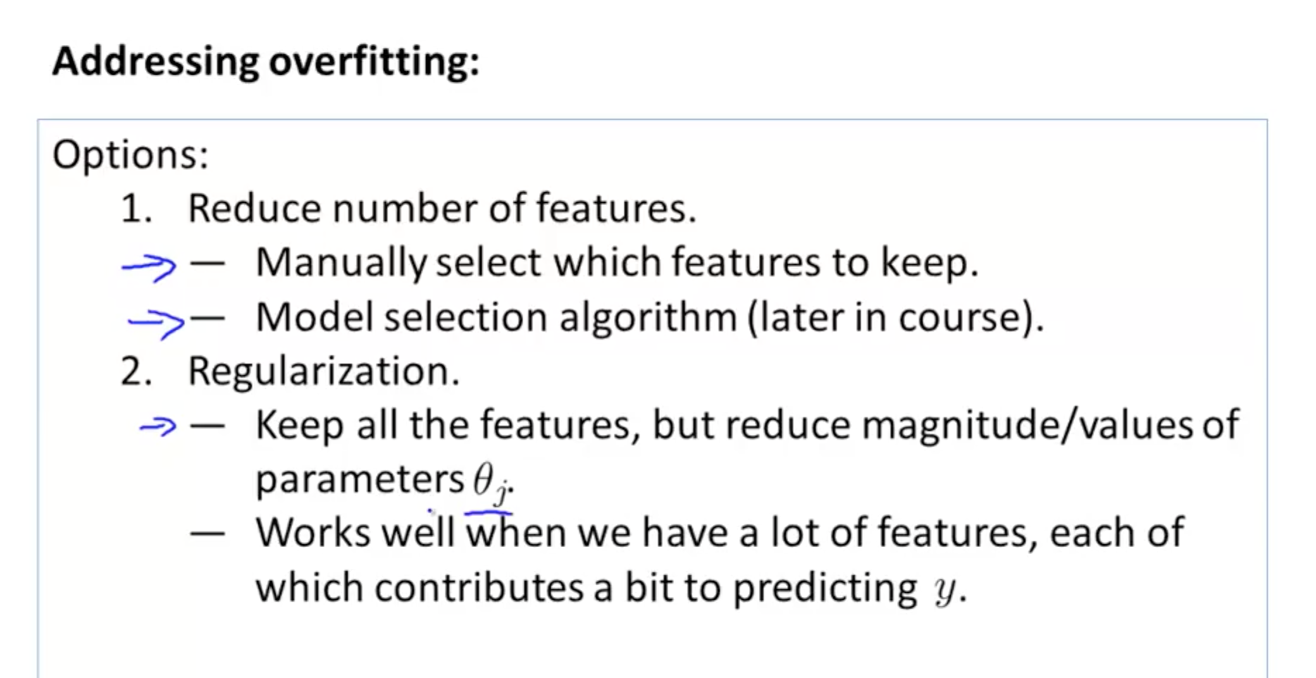
How to solve overfitting - Regularisation

Intuition of Regularisation - to make $\theta$ small

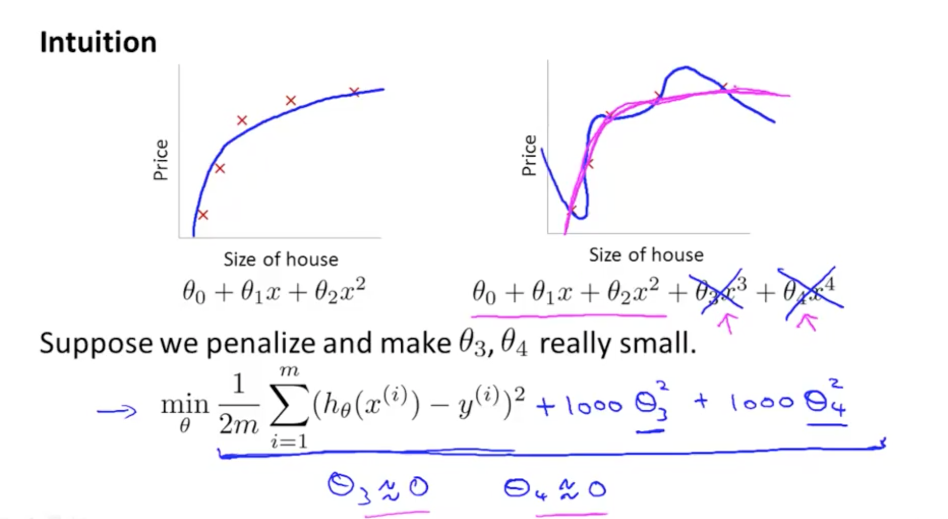
Shrink all the parameters - starts from $\theta_1$ not from $\theta_0$:

$$J(\theta)=\frac{1}{2m}[\sum^{m}_{i=1}(h_\theta(x^{(i)})-y^{(i)})^2+\lambda\sum^{n}_{i=1}\theta_j^2]$$

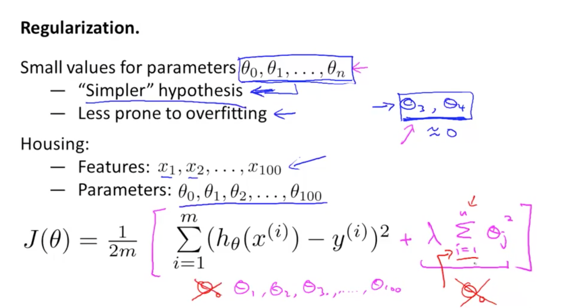
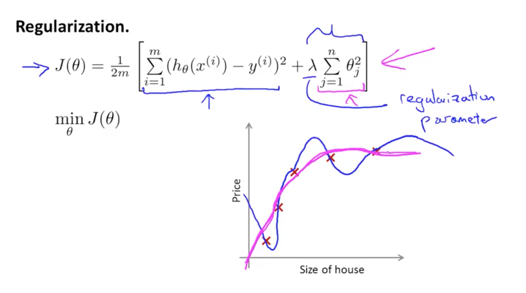
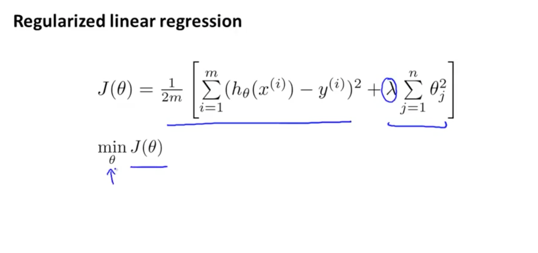
Regularisation Parameters

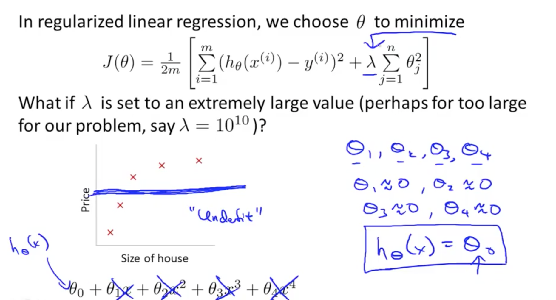
But the new parameter $\lambda$ used for regularisation can’t be too big otherwise will cause the all the $\theta$ too small (almost equals to 0) - underfitting

Cost Function and Gradient Descent With Regularization

Cost Function:

$$J(\theta)=\frac{1}{2m}[\sum^{m}_{i=1}(h_\theta(x^{(i)})-y^{(i)})^2+\lambda\sum^{n}_{i=1}\theta_j^2]$$

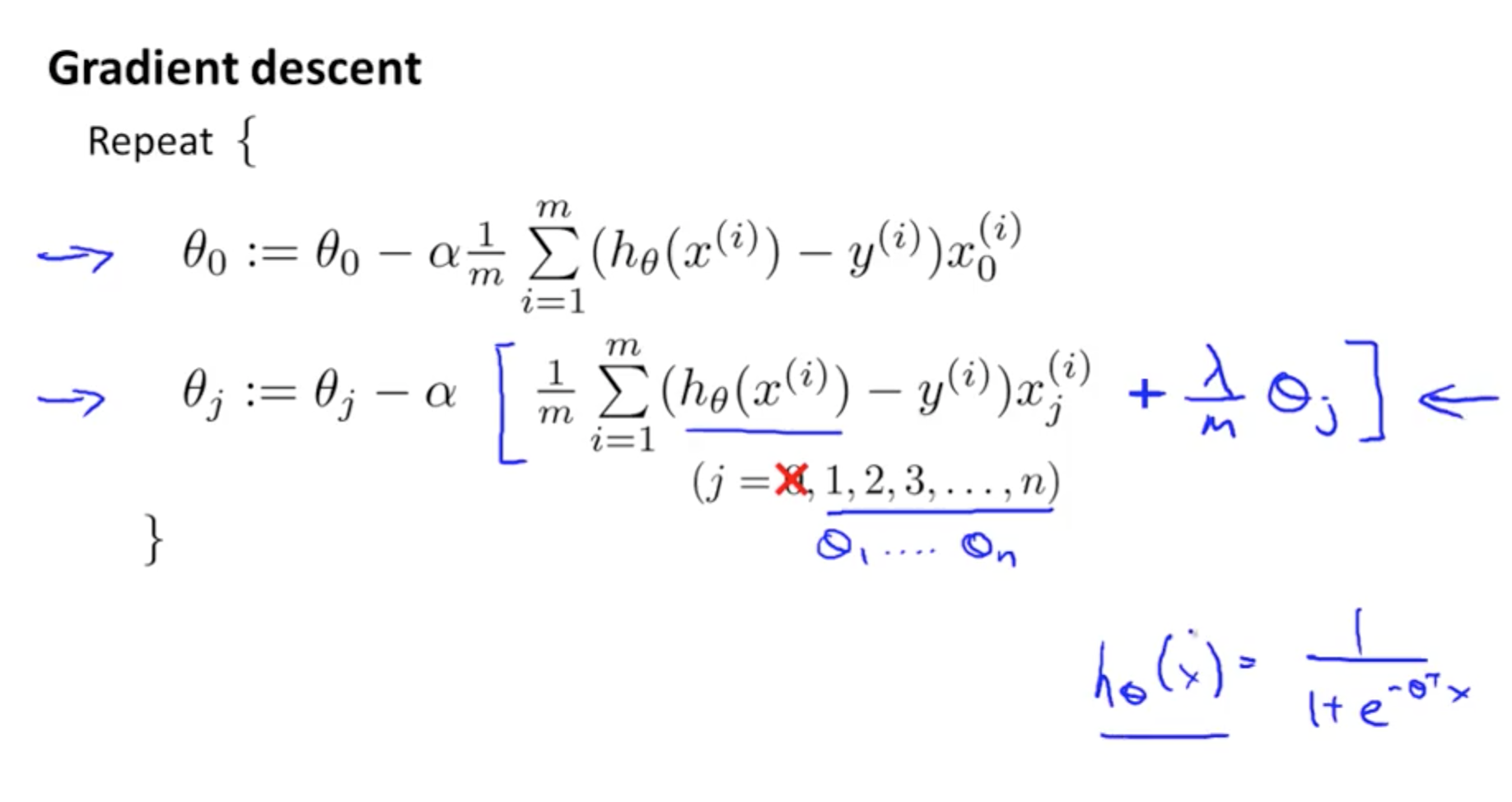
Gradient Descent:

$$\theta_0:=\theta_0-\alpha\frac1m\sum_{i=1}^m(h_\theta(x^{(i)})-y^{(i)})x_0^{(i)}$$
$$\theta_j:=\theta_j-\alpha[\frac1m\sum^m_{i=1}(h_\theta(x^{(i)})=y^{(i)})x_j^{(i)}+\frac\lambda m\theta_j (j=1,23...,n)$$

Normal Equation

The $\theta$ corresponding to global minimum:

$$\theta=(X^TX+\lambda \left[ \begin{matrix} 0 & 0 & 0 & ...\\ 0 & 1 & 0 & ...\\ 0 & 0 & 1 & ...\\ \end{matrix} \right] )^{-1}X^Ty$$

This will also make the original non-invertible matrix invertible

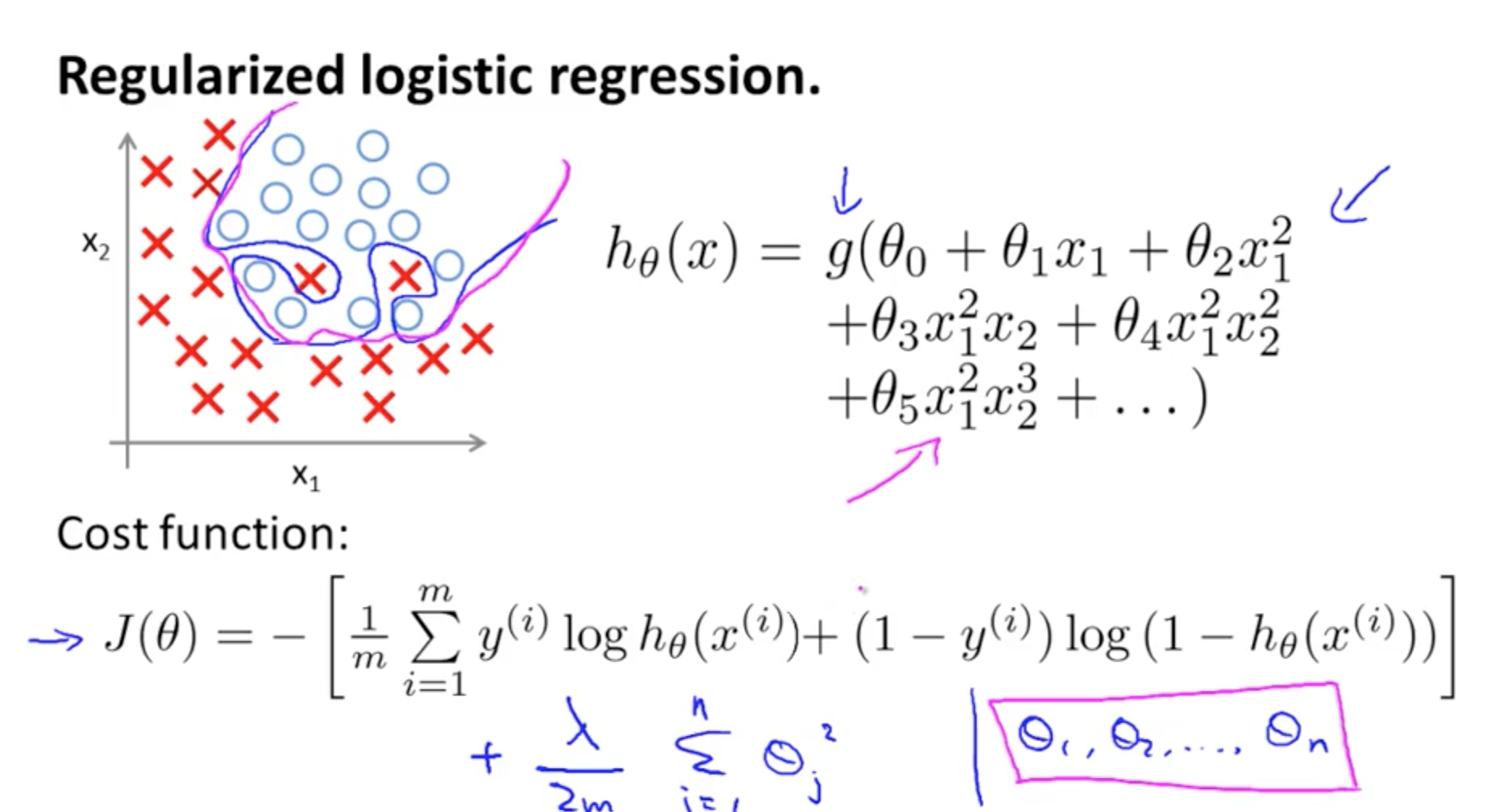
Regularized Logistic Regression

Cost Function:

$$J(\theta)=-[\frac1m\sum^m_{i=1}y^{(i)}log(h_\theta(x^{(i)}))+(1-y^{(i)})log(1-h_\theta(x^{(i)}))]+\frac{\lambda}{2m}\sum^n_{j=1}\theta_j^2$$

Repeating the Gradient Descent:

$$\theta_0:=\theta_0-\alpha\frac1m\sum^m_{i=1}(h_\theta(x^{(i)})-y^{(i)})x_o^{(i)}$$
$$\theta_j:=\theta_j-\alpha\frac1m\sum^m_{i=1}(h_\theta(x^{(i)})-y^{(i)})x_j^{(i)}+\frac{\lambda}m\theta_j$$
$$(j=1,2,3...),h_\theta(x)=\frac{1}{1+e^{-\theta^TX}}$$

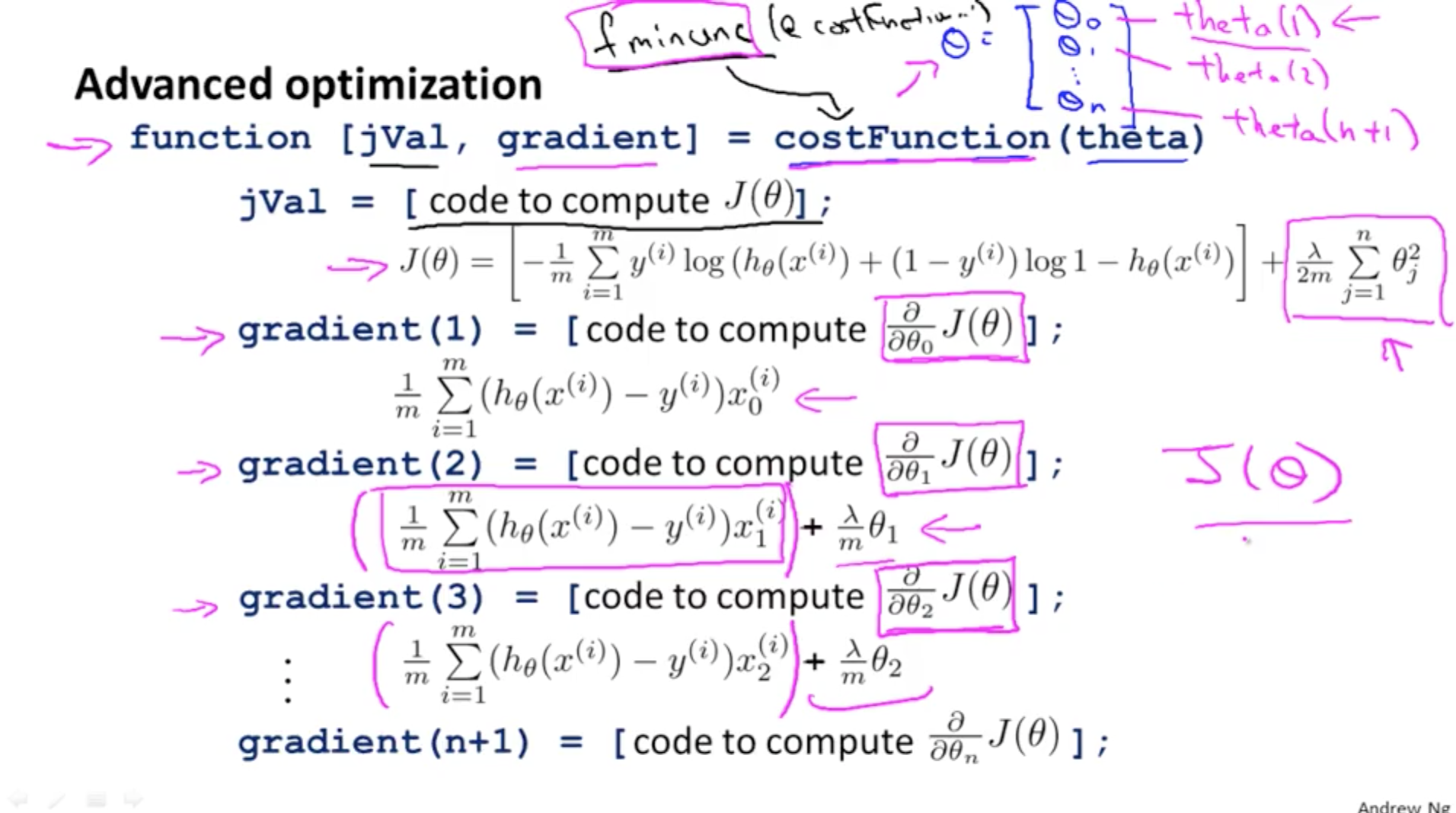
Matlab syntax:

fminunc(costFunction)

function[jVal,gradient]=costFunction(X,y,$\theta$)

Weekly Matlab Exercise

%sigmoid:

function g = sigmoid(z)
g = zeros(size(z));

g=1./(1+exp(-z))

end

%plotData:

function plotData(X, y)
figure; hold on;

pos=find(y==1);neg=find(y==0);
plot(X(pos,1),X(pos,2),'k+','LineWidth',2,'MarkerSize',7);
plot(X(neg,1),X(neg,2),'ko','MarkerFaceColor','y','MarkerSize',7);

hold off;
end

%costFunction(without regularisation):

function [J, grad] = costFunction(theta, X, y)
m = length(y); % number of training examples
J = 0;
grad = zeros(size(theta));

J=1/m*(-log(sigmoid(X*theta))'*y-log(1-sigmoid(X*theta))'*(1-y));
grad=1/m*((sigmoid(X*theta)-y)'*X)';

end

%predict:

function p = predict(theta, X)
m = size(X, 1); % Number of training examples
p = zeros(m, 1);

p=round(1./(1+exp(-X*theta)))

end

%costFunction(with regularisation):

function [J, grad] = costFunctionReg(theta, X, y, lambda)
m = length(y); % number of training examples
J = 0;
grad = zeros(size(theta));

theta2=theta(2:size(theta,1),1)
J=1/m*(-y'*log(sigmoid(X*theta))-(1.-y)'*log(1-sigmoid(X*theta)))+lambda./(2*m)*(theta2'*theta2)
grad1=(1/m*(sigmoid(X*theta)-y)'*X)'
theta1=lambda/m*theta
theta1(1,1)=0
grad=grad1+theta1

end

%use the fminunc function:

initial_theta = zeros(size(X, 2), 1);
% Set regularization parameter lambda to 1 (you should vary this)
lambda = 1;
% Set Options
options = optimset('GradObj', 'on', 'MaxIter', 400);
% Optimize
[theta, J, exit_flag] = ...
    fminunc(@(t)(costFunctionReg(t, X, y, lambda)), initial_theta, options);