Deep Leaning 学习笔记之改善神经网络的超参数（3.3）—— TensorFlow入门运行实例

最新推荐文章于 2022-08-26 21:18:38 发布

Aperact

最新推荐文章于 2022-08-26 21:18:38 发布

阅读量695

点赞数

分类专栏： DeepLearning TensorFlow

本文链接：https://blog.csdn.net/m0_37108127/article/details/98961736

版权

DeepLearning 同时被 2 个专栏收录

25 篇文章 3 订阅

订阅专栏

TensorFlow

1 篇文章 0 订阅

订阅专栏

1 TensorFlow框架

有许多机器学习的框架，可以减少代码量，并且能够自动执行例如梯度下降函数等，加快程序的运行速度，TensorFlow就是众多框架中的一种

在这里插入图片描述

1.1 TensorFlow步骤

在TensorFlow中编写和运行程序的步骤如下:

创建尚未执行/计算的张量(变量)——variables
写出这些张量之间的运算。
初始化你的张量。
创建一个会话。
运行会话。这将运行上面所写的操作。
因此，当我们为损失创建一个变量时，我们简单地将损失定义为其他量的函数，但没有计算它的值。为了计算它，我们必须运行
init=tf.global_variables_initializer()
初始化了loss变量，最后一行我们终于能够计算loss的值并打印它的值。
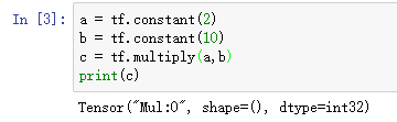
现在让我们看一个简单的例子。运行以下单元格:

1.2 分步介绍

1.2.1 sess的重要性

在这里插入图片描述
这是由于我把它放入“计算图”中，但是还没有运行这个计算。
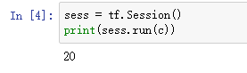
为了将这两个数字相乘，必须创建一个会话并运行它。
如下：

总之，请记住初始化变量、创建会话并在会话中运行操作。

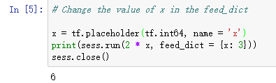
1.2.2 placeholders占位符

placeholders是一个对象，您只能在稍后指定其值。要为placeholders指定值，可以使用"feed dictionary"（提要字典）(feed_dict变量)传入值。
在这里插入图片描述
当您第一次定义x时，您不必为它指定值。占位符只是一个变量，您只会在稍后运行会话时将数据分配给该变量。我们说您在运行会话时将数据提供给这些占位符。
事情是这样的:当您指定一个计算所需的操作时，您是在告诉TensorFlow如何构造一个计算图。计算图可以有一些占位符，稍后您将指定这些占位符的值。最后，当您运行会话时，您告诉TensorFlow执行计算图。

2 TensorFlow练习

2.1 线性方程

Compute $W X + b$ $W, X$ , and $b$ 是随机正态分布。
W is of shape (4, 3), X is (3,1) and b is (4,1).
定义shape为（3,1）的常量X语句如下：

X = tf.constant(np.random.randn(3,1), name = "X")

tf.matmul(…, …)代表矩阵相乘
tf.add(…, …)代表做加法
np.random.randn(…)代表随机初始化

# GRADED FUNCTION: linear_function

def linear_function():
    """
    Implements a linear function: 
            Initializes W to be a random tensor of shape (4,3)
            Initializes X to be a random tensor of shape (3,1)
            Initializes b to be a random tensor of shape (4,1)
    Returns: 
    result -- runs the session for Y = WX + b 
    """
    
    np.random.seed(1)
    
    ### START CODE HERE ### (4 lines of code)
    X = tf.constant(np.random.randn(3,1), name = "X")
    W = tf.constant(np.random.randn(4,3), name = "W")
    b = tf.constant(np.random.randn(4,1), name = "b")
    Y = tf.add(tf.matmul(W, X),b)
    ### END CODE HERE ### 
    
    # Create the session using tf.Session() and run it with sess.run(...) on the variable you want to calculate
    
    ### START CODE HERE ###
    sess = tf.Session()
    result = sess.run(Y)
    ### END CODE HERE ### 
    
    # close the session 
    sess.close()

    return result

在这里插入图片描述

2.2 Sigmoid

您将使用占位符变量x来做这个练习。当运行会话时，您应该使用提要字典来传入输入z。
在这个练习中，您必须

创建一个占位符x
定义使用tf计算sigmoid所需的操作
运行会话。

练习：实现下面的sigmoid函数。你应该使用以下方法:

tf.placeholder(tf.float32, name = "...")
tf.sigmoid(...)
sess.run(..., feed_dict = {x: z})

注意，在tensorflow中有两种创建和使用会话的典型方法:

Method 1:

sess = tf.Session()
# Run the variables initialization (if needed), run the operations
result = sess.run(..., feed_dict = {...})
sess.close() # Close the session

Method 2:

with tf.Session() as sess: 
    # run the variables initialization (if needed), run the operations
    result = sess.run(..., feed_dict = {...})
    # This takes care of closing the session for you :)

# GRADED FUNCTION: sigmoid

def sigmoid(z):
    """
    Computes the sigmoid of z
    
    Arguments:
    z -- input value, scalar or vector
    
    Returns: 
    results -- the sigmoid of z
    """
    
    ### START CODE HERE ### ( approx. 4 lines of code)
    # Create a placeholder for x. Name it 'x'.
    x = tf.placeholder(tf.float32, name = "x")

    # compute sigmoid(x)
    sigmoid =  1/(1+math.e**-x) 

    # Create a session, and run it. Please use the method 2 explained above. 
    # You should use a feed_dict to pass z's value to x. 
    with tf.Session() as sess:
        # Run session and call the output "result"
        result = sess.run(sigmoid,feed_dict={x:z})
    
    ### END CODE HERE ###
    
    return result

在这里插入图片描述

2.3 计算cost（逻辑回归）

现在不需要写一长串代码来计算逻辑回归函数
$\frac{1}{m} \sum_{i = 1}^m \large ( \small y^{(i)} \log a^{ [2] (i)} + (1-y^{(i)})\log (1-a^{ [2] (i)} )\large )\small\tag{2}$
只需要用以下语句即可

tf.nn.sigmoid_cross_entropy_with_logits(logits = ..., labels = ...)

# GRADED FUNCTION: cost

def cost(logits, labels):
    """
    Computes the cost using the sigmoid cross entropy
    
    Arguments:
    logits -- vector containing z, output of the last linear unit (before the final sigmoid activation)
    labels -- vector of labels y (1 or 0) 
    
    Note: What we've been calling "z" and "y" in this class are respectively called "logits" and "labels" 
    in the TensorFlow documentation. So logits will feed into z, and labels into y. 
    
    Returns:
    cost -- runs the session of the cost (formula (2))
    """
    
    ### START CODE HERE ### 
    
    # Create the placeholders for "logits" (z) and "labels" (y) (approx. 2 lines)
    z = tf.placeholder(tf.float32, name = "z")
    y = tf.placeholder(tf.float32, name = "y")
    
    # Use the loss function (approx. 1 line)
    cost = tf.nn.sigmoid_cross_entropy_with_logits(logits = z,  labels = y)
    
    # Create a session (approx. 1 line). See method 1 above.
    sess = tf.Session()
    
    # Run the session (approx. 1 line).
    cost = sess.run(cost,feed_dict = {z:logits,y:labels})
    
    # Close the session (approx. 1 line). See method 1 above.
    sess.close()
    
    ### END CODE HERE ###
    
    return cost

在这里插入图片描述

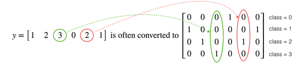
2.4 使用One Hot 编码

当C = N时（此例为4），要进行y的转换，就需要用到One Hot编码

tf.one_hot(labels, depth, axis)

# GRADED FUNCTION: cost

def cost(logits, labels):
    """
    Computes the cost using the sigmoid cross entropy
    
    Arguments:
    logits -- vector containing z, output of the last linear unit (before the final sigmoid activation)
    labels -- vector of labels y (1 or 0) 
    
    Note: What we've been calling "z" and "y" in this class are respectively called "logits" and "labels" 
    in the TensorFlow documentation. So logits will feed into z, and labels into y. 
    
    Returns:
    cost -- runs the session of the cost (formula (2))
    """
    
    ### START CODE HERE ### 
    
    # Create the placeholders for "logits" (z) and "labels" (y) (approx. 2 lines)
    z = tf.placeholder(tf.float32, name = "z")
    y = tf.placeholder(tf.float32, name = "y")
    
    # Use the loss function (approx. 1 line)
    cost = tf.nn.sigmoid_cross_entropy_with_logits(logits = z,  labels = y)
    
    # Create a session (approx. 1 line). See method 1 above.
    sess = tf.Session()
    
    # Run the session (approx. 1 line).
    cost = sess.run(cost,feed_dict = {z:logits,y:labels})
    
    # Close the session (approx. 1 line). See method 1 above.
    sess.close()
    
    ### END CODE HERE ###
    
    return cost

在这里插入图片描述

2.5 0-1初始化

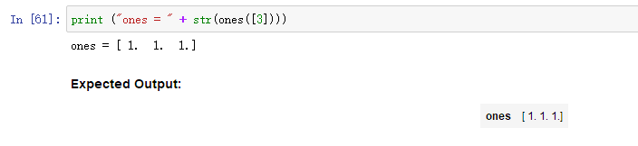
现在您将学习如何初始化一个由0和1组成的向量。您将调用的函数是tf.ones()。要用0初始化，可以使用tf.zeros()。这些函数呈现一个形状，并分别返回一个包含0和1的维度形状数组。

tf.ones(shape)

# GRADED FUNCTION: ones

def ones(shape):
    """
    Creates an array of ones of dimension shape
    
    Arguments:
    shape -- shape of the array you want to create
        
    Returns: 
    ones -- array containing only ones
    """
    
    ### START CODE HERE ###
    
    # Create "ones" tensor using tf.ones(...). (approx. 1 line)
    ones = tf.ones(shape)
    
    # Create the session (approx. 1 line)
    sess = tf.Session()
    
    # Run the session to compute 'ones' (approx. 1 line)
    ones = sess.run(ones)
    
    # Close the session (approx. 1 line). See method 1 above.
    sess.close()
    
    ### END CODE HERE ###
    return ones

在这里插入图片描述

3 建立神经网络（使用TensorFlow）

在这部分作业中，您将使用tensorflow构建一个神经网络。记住，实现tensorflow模型有两部分:

创建计算图
运行图表

3.1 数据预处理

将数据扁平化（一个样本为一列）
数据标准化（/255）
处理标签Y为hot矩阵
在这里插入图片描述

3.2 X,Y创建占位符

# GRADED FUNCTION: create_placeholders

def create_placeholders(n_x, n_y):
    """
    Creates the placeholders for the tensorflow session.
    
    Arguments:
    n_x -- scalar, size of an image vector (num_px * num_px = 64 * 64 * 3 = 12288)
    n_y -- scalar, number of classes (from 0 to 5, so -> 6)
    
    Returns:
    X -- placeholder for the data input, of shape [n_x, None] and dtype "float"
    Y -- placeholder for the input labels, of shape [n_y, None] and dtype "float"
    
    Tips:
    - You will use None because it let's us be flexible on the number of examples you will for the placeholders.
      In fact, the number of examples during test/train is different.
    """

    ### START CODE HERE ### (approx. 2 lines)
    X = tf.placeholder(tf.float32, shape=(n_x, None),name = "X")
    Y = tf.placeholder(tf.float32, shape=(n_y, None),name = "Y")
    ### END CODE HERE ###
    
    return X, Y

在这里插入图片描述

3.3 初始化参数

# GRADED FUNCTION: initialize_parameters

def initialize_parameters():
    """
    Initializes parameters to build a neural network with tensorflow. The shapes are:
                        W1 : [25, 12288]
                        b1 : [25, 1]
                        W2 : [12, 25]
                        b2 : [12, 1]
                        W3 : [6, 12]
                        b3 : [6, 1]
    
    Returns:
    parameters -- a dictionary of tensors containing W1, b1, W2, b2, W3, b3
    """
    
    tf.set_random_seed(1)                   # so that your "random" numbers match ours
        
    ### START CODE HERE ### (approx. 6 lines of code)
    W1 = tf.get_variable("W1", [25,12288], initializer = tf.contrib.layers.xavier_initializer(seed = 1))
    b1 = tf.get_variable("b1", [25,1], initializer = tf.zeros_initializer())
    W2 = tf.get_variable("W2", [12,25], initializer = tf.contrib.layers.xavier_initializer(seed = 1))
    b2 = tf.get_variable("b2", [12,1], initializer = tf.zeros_initializer())
    W3 = tf.get_variable("W3", [6,12], initializer = tf.contrib.layers.xavier_initializer(seed = 1))
    b3 = tf.get_variable("b3", [6,1], initializer = tf.zeros_initializer())
    ### END CODE HERE ###

    parameters = {"W1": W1,
                  "b1": b1,
                  "W2": W2,
                  "b2": b2,
                  "W3": W3,
                  "b3": b3}
    
    return parameters

在这里插入图片描述

3.4 Forward propagation in tensorflow

现在，您将在tensorflow中实现正向传播模块。该函数将接受一个参数字典，并完成向前传递。你将使用的功能是:

tf.add(...,...) to do an addition
tf.matmul(...,...) to do a matrix multiplication
tf.nn.relu(...) to apply the ReLU activation

注意！！！！

实现了神经网络的正向传递。我们为您注释了numpy等价物，以便您可以将tensorflow实现与numpy进行比较。
需要注意的是，正向传播在z3处停止。
原因是，最后一个线性层的输出作为计算损耗的函数的输入（也就是把Z3当做input去计算SOFTMAX.）。因此，您不需要a3!

# GRADED FUNCTION: forward_propagation

def forward_propagation(X, parameters):
    """
    Implements the forward propagation for the model: LINEAR -> RELU -> LINEAR -> RELU -> LINEAR -> SOFTMAX
    
    Arguments:
    X -- input dataset placeholder, of shape (input size, number of examples)
    parameters -- python dictionary containing your parameters "W1", "b1", "W2", "b2", "W3", "b3"
                  the shapes are given in initialize_parameters

    Returns:
    Z3 -- the output of the last LINEAR unit
    """
    
    # Retrieve the parameters from the dictionary "parameters" 
    W1 = parameters['W1']
    b1 = parameters['b1']
    W2 = parameters['W2']
    b2 = parameters['b2']
    W3 = parameters['W3']
    b3 = parameters['b3']
    
    ### START CODE HERE ### (approx. 5 lines)                                     # Numpy Equivalents:
    Z1 = tf.add(tf.matmul(W1,X),b1)                                               # Z1 = np.dot(W1, X) + b1
    A1 = tf.nn.relu(Z1)                                                           # A1 = relu(Z1)
    Z2 = tf.add(tf.matmul(W2,A1),b2)                                              # Z2 = np.dot(W2, a1) + b2
    A2 = tf.nn.relu(Z2)                                                           # A2 = relu(Z2)
    Z3 = tf.add(tf.matmul(W3,A2),b3)                                              # Z3 = np.dot(W3,A2) + b3
    ### END CODE HERE ###
    
    return Z3

在这里插入图片描述
您可能已经注意到正向传播不输出任何缓存。下面，当我们讲到brackpropagation时，您将理解其中的原因。

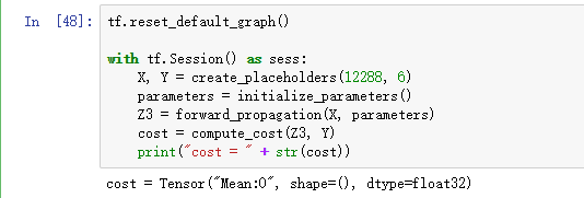
3.5 计算Cost

使用如下函数计算Cost

tf.reduce_mean(tf.nn.softmax_cross_entropy_with_logits(logits = ..., labels = ...))

# GRADED FUNCTION: compute_cost 

def compute_cost(Z3, Y):
    """
    Computes the cost
    
    Arguments:
    Z3 -- output of forward propagation (output of the last LINEAR unit), of shape (6, number of examples)
    Y -- "true" labels vector placeholder, same shape as Z3
    
    Returns:
    cost - Tensor of the cost function
    """
    
    # to fit the tensorflow requirement for tf.nn.softmax_cross_entropy_with_logits(...,...)
    logits = tf.transpose(Z3)
    labels = tf.transpose(Y)
    
    ### START CODE HERE ### (1 line of code)
    cost = tf.reduce_mean(tf.nn.softmax_cross_entropy_with_logits(logits=logits ,labels=labels ))
    ### END CODE HERE ###
    
    return cost

在这里插入图片描述

3.6 反向传播和参数更新

计算成本函数之后。您将创建一个“优化器”对象。在运行tf.session时，您必须调用这个对象以及成本。当调用时，它将使用所选择的方法和学习率对给定的成本进行优化。

例如，对于梯度下降，优化器将是:

optimizer = tf.train.GradientDescentOptimizer(learning_rate = learning_rate).minimize(cost)

要进行优化，你需要:

_ , c = sess.run([optimizer, cost], feed_dict={X: minibatch_X, Y: minibatch_Y})

在编码时，我们经常使用_作为“一次性”变量来存储我们以后不需要使用的值。这里，_接受优化器的评估值，我们不需要它(而c接受成本变量的值)。

3.7 总体Model建立

def model(X_train, Y_train, X_test, Y_test, learning_rate = 0.0001,
          num_epochs = 1500, minibatch_size = 32, print_cost = True):
    """
    Implements a three-layer tensorflow neural network: LINEAR->RELU->LINEAR->RELU->LINEAR->SOFTMAX.
    
    Arguments:
    X_train -- training set, of shape (input size = 12288, number of training examples = 1080)
    Y_train -- test set, of shape (output size = 6, number of training examples = 1080)
    X_test -- training set, of shape (input size = 12288, number of training examples = 120)
    Y_test -- test set, of shape (output size = 6, number of test examples = 120)
    learning_rate -- learning rate of the optimization
    num_epochs -- number of epochs of the optimization loop
    minibatch_size -- size of a minibatch
    print_cost -- True to print the cost every 100 epochs
    
    Returns:
    parameters -- parameters learnt by the model. They can then be used to predict.
    """
    
    ops.reset_default_graph()                         # to be able to rerun the model without overwriting tf variables
    tf.set_random_seed(1)                             # to keep consistent results
    seed = 3                                          # to keep consistent results
    (n_x, m) = X_train.shape                          # (n_x: input size, m : number of examples in the train set)
    n_y = Y_train.shape[0]                            # n_y : output size
    costs = []                                        # To keep track of the cost
    
    # Create Placeholders of shape (n_x, n_y)
    ### START CODE HERE ### (1 line)
    X, Y = create_placeholders(n_x, n_y)
    ### END CODE HERE ###

    # Initialize parameters
    ### START CODE HERE ### (1 line)
    parameters = initialize_parameters()
    ### END CODE HERE ###
    
    # Forward propagation: Build the forward propagation in the tensorflow graph
    ### START CODE HERE ### (1 line)
    Z3 = forward_propagation(X, parameters)
    ### END CODE HERE ###
    
    # Cost function: Add cost function to tensorflow graph
    ### START CODE HERE ### (1 line)
    cost = compute_cost(Z3, Y)
    ### END CODE HERE ###
    
    # Backpropagation: Define the tensorflow optimizer. Use an AdamOptimizer.
    ### START CODE HERE ### (1 line)
    optimizer =  tf.train.AdamOptimizer(learning_rate = learning_rate).minimize(cost)
    ### END CODE HERE ###
    
    # Initialize all the variables
    init = tf.global_variables_initializer()

    # Start the session to compute the tensorflow graph
    with tf.Session() as sess:
        
        # Run the initialization
        sess.run(init)
        
        # Do the training loop
        for epoch in range(num_epochs):

            epoch_cost = 0.                       # Defines a cost related to an epoch
            num_minibatches = int(m / minibatch_size) # number of minibatches of size minibatch_size in the train set
            seed = seed + 1
            minibatches = random_mini_batches(X_train, Y_train, minibatch_size, seed)

            for minibatch in minibatches:

                # Select a minibatch
                (minibatch_X, minibatch_Y) = minibatch
                
                # IMPORTANT: The line that runs the graph on a minibatch.
                # Run the session to execute the "optimizer" and the "cost", the feedict should contain a minibatch for (X,Y).
                ### START CODE HERE ### (1 line)
                _ , minibatch_cost = sess.run([optimizer, cost], feed_dict={X: minibatch_X, Y: minibatch_Y})
                ### END CODE HERE ###
                
                epoch_cost += minibatch_cost / num_minibatches

            # Print the cost every epoch
            if print_cost == True and epoch % 100 == 0:
                print ("Cost after epoch %i: %f" % (epoch, epoch_cost))
            if print_cost == True and epoch % 5 == 0:
                costs.append(epoch_cost)
                
        # plot the cost
        plt.plot(np.squeeze(costs))
        plt.ylabel('cost')
        plt.xlabel('iterations (per tens)')
        plt.title("Learning rate =" + str(learning_rate))
        plt.show()

        # lets save the parameters in a variable
        parameters = sess.run(parameters)
        print ("Parameters have been trained!")

        # Calculate the correct predictions
        correct_prediction = tf.equal(tf.argmax(Z3), tf.argmax(Y))

        # Calculate accuracy on the test set
        accuracy = tf.reduce_mean(tf.cast(correct_prediction, "float"))

        print ("Train Accuracy:", accuracy.eval({X: X_train, Y: Y_train}))
        print ("Test Accuracy:", accuracy.eval({X: X_test, Y: Y_test}))
        
        return parameters

在这里插入图片描述

4 总结

您应该记住的是:
创建一个包含张量(变量、占位符……)和操作(tf)的图。matmul,特遣部队。添加、…)创建会话初始化会话运行会话以执行图您可以多次执行图，正如您在model()中看到的那样，当在“优化器”对象上运行会话时，会自动执行反向传播和优化。

What you should remember:

Tensorflow是一个用于深度学习的编程框架
Tensorflow中的两个主要对象类是Tensors（张量）和Operators（操作符）。
在tensorflow中编写代码时，必须执行以下步骤:
- 创建一个图graph，包含 Tensors (Variables, Placeholders …) 和 Operations (tf.matmul, tf.add, …)
- 建立一个 session
- 初始化 session
- 通过执行会话来执行图 graph
图 graph 可以多次执行
当在“优化器”对象上运行会话时，会自动执行反向传播和优化

Aperact

关注

0
点赞
踩
0

收藏

觉得还不错? 一键收藏
0
评论
Deep Leaning 学习笔记之改善神经网络的超参数（3.3）—— TensorFlow入门运行实例

1 TensorFlow框架有许多机器学习的框架，可以减少代码量，并且能够自动执行例如梯度下降函数等，加快程序的运行速度，TensorFlow就是众多框架中的一种1.1 TensorFlow步骤在TensorFlow中编写和运行程序的步骤如下:创建尚未执行/计算的张量(变量)——variables写出这些张量之间的运算。初始化你的张量。创建一个会话。运行会话。这将运行上面所写...
复制链接

扫一扫