（五）循环神经网络 -- 4 循环神经网络的实现

4. 循环神经网络的实现

import numpy as np
import tensorflow as tf
print(tf.__version__)

# 将「语言模型数据集」一节中的代码封装至d2lzh_tensorflow2中
import d2lzh_tensorflow2 as d2l

2.0.0

4.1 定义模型

4.1.1 RNN模块

Keras的RNN模块提供了循环神经网络的实现。

构造一个含单隐藏层、隐藏单元个数为256的循环神经网络层rnn_layer，并对权重做初始化。代码示例如下：

num_hiddens = 256
cell = tf.keras.layers.SimpleRNNCell(units=num_hiddens, kernel_initializer='glorot_uniform')

"""
tf.keras.layers.RNN:
    cell: A RNN cell instance or a list of RNN cell instances. A RNN cell is a class that has:
        A call(input_at_t, states_at_t) method, returning (output_at_t, states_at_t_plus_1). 
        A state_size attribute. 
        A output_size attribute. 
        A get_initial_state(inputs=None, batch_size=None, dtype=None) method that creates a tensor meant to be fed to call() as the initial state, if the user didn't specify any initial state via other means. 
"""
rnn_layer = tf.keras.layers.RNN(cell, return_sequences=True, return_state=True, time_major=True)

其中，rnn_layer的输入形状为(时间步数, 批量大小, 输入个数)。
输入个数，即one-hot向量长度（词典大小）。

此外，rnn_layer在前向计算后会分别返回输出和隐藏状态h。
输出指隐藏层在各个时间步上计算并输出的隐藏状态，它们通常作为后续输出层的输入。需要强调的是，该“输出”本身并不涉及输出层计算，形状为(时间步数, 批量大小, 隐藏单元个数)；
隐藏状态指隐藏层在最后时间步的隐藏状态。当隐藏层有多层时，每一层的隐藏状态都会记录在该变量中。对于如长短期记忆（LSTM），隐藏状态是一个元组(h, c)，即hidden state和cell state。

关于循环神经网络（以LSTM为例）的输出，图示如下：

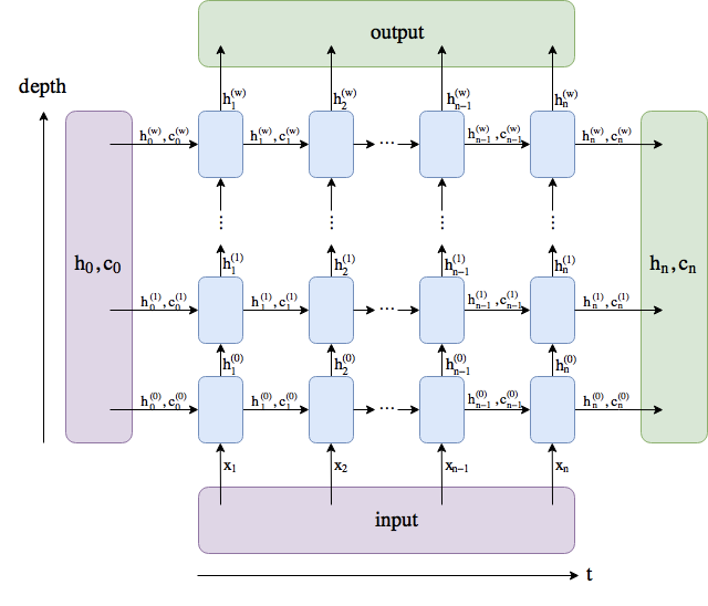
对于rnn_layer，输出形状为(时间步数, 批量大小, 隐藏单元个数)，隐藏状态h的形状为(层数, 批量大小, 隐藏单元个数)，有：

def load_data_jay_lyrics():

    """
    得到上一节所示的变量
    """     
    
    with open('jaychou_lyrics.txt') as f:
        corpus_chars = f.read()

    corpus_chars = corpus_chars.replace('\n', ' ').replace('\r', ' ')
    corpus_chars = corpus_chars[:10000]

    idx_to_char = list(set(corpus_chars))
    char_to_idx = {v:k for k,v in enumerate(idx_to_char)}
    vocab_size = len(char_to_idx)
    
    corpus_indices = [char_to_idx[char] for char in corpus_chars]

    return corpus_indices, char_to_idx, idx_to_char, vocab_size

(corpus_indices, char_to_idx, idx_to_char, vocab_size) = load_data_jay_lyrics()

batch_size = 2
state = cell.get_initial_state(batch_size=batch_size,dtype=tf.float32)

num_steps = 35
X = tf.random.uniform(shape=(num_steps, batch_size, vocab_size))

# return_state=True
Y, state_new = rnn_layer(X, state)

Y.shape, len(state_new), state_new[0].shape

输出：

(TensorShape([35, 2, 256]), 2, TensorShape([256]))

4.1.2 继承Module类

one-hot向量

为了将词表示为向量输入到神经网络，一个简单的办法是使用one-hot向量。

假设词典中不同字符的数量为$N$（即，词典大小vocab_size），每个字符已与从0到$N-1$的连续整数值索引一一对应。
若一个字符的索引为整数$i$，那么创建一个全0的长为$N$的向量，并将其位置为$i$的元素设成1。该向量就是对原字符的one-hot向量。

索引为0和2的one-hot向量（向量长度等于词典大小），示例如下：

tf.one_hot(np.array([0, 2]), vocab_size)

输出：

<tf.Tensor: id=526, shape=(2, 1027), dtype=float32, numpy=
array([[1., 0., 0., ..., 0., 0., 0.],
       [0., 0., 1., ..., 0., 0., 0.]], dtype=float32)>

模型定义

通过继承Module类来定义一个完整的循环神经网络。

先将输入数据使用one-hot向量表示并输入到rnn_layer中，再使用全连接输出层得到输出（输出个数等于词典大小vocab_size），代码示例如下：

class RNNModel(tf.keras.layers.Layer):
    def __init__(self, rnn_layer, vocab_size, **kwargs):
        super(RNNModel, self).__init__(**kwargs)
        self.rnn = rnn_layer
        self.vocab_size = vocab_size
        self.dense = tf.keras.layers.Dense(units=vocab_size)
        
    def call(self, inputs, state):
        """
        tf.one_hot:
            indices = [[0, 2], [1, -1]]
            depth = 3
            tf.one_hot(indices, depth,
                       on_value=1.0, off_value=0.0,
                       axis=-1)  # output: [2 x 2 x 3]
            # [[[1.0, 0.0, 0.0],   # one_hot(0)
            #   [0.0, 0.0, 1.0]],  # one_hot(2)
            #  [[0.0, 1.0, 0.0],   # one_hot(1)
            #   [0.0, 0.0, 0.0]]]  # one_hot(-1)
        """
        # 将输入转置为(num_steps, batch_size)，再进行one-hot向量表示
        X = tf.one_hot(indices=tf.transpose(inputs), depth=self.vocab_size)
        Y, state = self.rnn(X, state)
        
        # Y先reshape to (num_steps * batch_size, num_hiddens)，再过dense层
        # 最终输出形状: (num_steps * batch_size, vocab_size)
        output = self.dense(tf.reshape(Y, shape=(-1, Y.shape[-1])))
        return output, state
    
    def get_initial_state(self, *args, **kwargs):
        return self.rnn.cell.get_initial_state(*args, **kwargs)

4.2 训练模型

基于前缀prefix（含有数个字符的字符串）来预测接下来的num_chars个字符。

4.2.1 预测函数

定义一个预测函数，代码示例如下：

def predict_rnn_keras(prefix, num_chars, model, vocab_size, idx_to_char, char_to_idx):
    
    """
    tf.argmax:
        Returns the index with the largest value across axes of a tensor.
        B=tf.constant([[2,20,30,3,6],[3,11,16,1,8],[14,45,23,5,27]])
        tf.argmax(B,axis=0) # [2, 2, 0, 2, 2]
        tf.argmax(B,axis=1) # [2, 2, 1]
        tf.argmax(B,axis=-1) # [2, 2, 1]
    """
    
    # 使用model的成员函数来初始化隐藏状态
    state = model.get_initial_state(batch_size=1, dtype=tf.float32)
    output = [char_to_idx[prefix[0]]]
    
    for t in range(len(prefix)+num_chars-1):
        X = np.array([output[-1]]).reshape((1, 1))
        Y, state = model(X, state)
        
        if t < len(prefix)-1:
            output.append(char_to_idx[prefix[t+1]])
        else:
            # 取Y中max值
            output.append(int(np.array(tf.argmax(Y, axis=-1))))
            
    return ''.join([idx_to_char[i] for i in output])

根据前缀“分开”，创作长度为10个字符（不考虑前缀长度）的一段歌词。使用权重为随机值的模型来进行一次预测，代码示例如下：

model = RNNModel(rnn_layer, vocab_size)
predict_rnn_keras('分开', 10, model, vocab_size,  idx_to_char, char_to_idx)

输出：

'分开言龙印颁悲杂回词悉逃'

因为模型参数为随机值，所以预测结果也为随机。

4.2.2 模型训练

裁剪梯度

循环神经网络中，较容易出现梯度衰减或梯度爆炸（将在下一小节解释原因）。

为了应对梯度爆炸，可以裁剪梯度（clip gradient）。假设把所有模型参数梯度的元素拼接成一个向量 $\mathbf{g}$，裁剪的阈值为$\theta$，那么，有：

$$\min \left(\frac{\theta }{||\mathbf{g}||},1\right)\mathbf{g}$$

其中，裁剪后梯度的$L_2$范数不超过$\theta$。

计算裁剪后的梯度，代码示例如下：

def grad_clipping(grads, theta):
    norm = np.array([0])
    for i in range(len(grads)):
        norm += tf.reduce_sum(grads[i]**2)
    norm = np.sqrt(norm).item()
    
    new_gradients = []
    if norm > theta:
        for grad in grads:
            new_gradients.append(grad*theta/norm)
    else:
        for grad in grads:
            new_gradients.append(grad)
    return new_gradients

困惑度

通常使用困惑度（perplexity）来评价语言模型的好坏。结合 softmax回归 小节中交叉熵损失函数的定义，困惑度是对交叉熵损失函数做指数运算后得到的值。

特别地，
最佳情况下，模型总是把标签类别的概率预测为1，此时困惑度为1；
最坏情况下，模型总是把标签类别的概率预测为0，此时困惑度为正无穷；
基线情况下，模型总是预测所有类别的概率都相同，此时困惑度为类别个数。

显然，任何一个有效模型的困惑度必须小于类别个数。
在本例中，困惑度必须小于词典大小vocab_size。

模型训练

训练函数使用了相邻采样来读取数据：

def train_and_predict_rnn_keras(model, num_hiddens, vocab_size, 
                                corpus_indices, idx_to_char, char_to_idx,
                                num_epochs, num_steps, lr, clipping_theta,
                                batch_size, pred_period, pred_len, prefixes):
    """
    SparseCategoricalCrossentropy vs sparse_categorical_crossentropy:

        https://stackoverflow.com/questions/58565394/what-is-the-difference-between-sparse-categorical-crossentropy-and-categorical-c

        categorical_crossentropy (cce) uses a one-hot array to calculate the probability,
        sparse_categorical_crossentropy (scce) uses a category index

    """
    
    import time
    import math
    
    loss = tf.keras.losses.SparseCategoricalCrossentropy()
    optimizer = tf.keras.optimizers.SGD(learning_rate=lr)
    
    for epoch in range(num_epochs):
        l_sum, n, start = 0.0, 0, time.time()
        # 相邻采样
        data_iter = d2l.data_iter_consecutive(corpus_indices, batch_size, num_steps)
        state = model.get_initial_state(batch_size=batch_size, dtype=tf.float32)
        
        for X, Y in data_iter:
            with tf.GradientTape(persistent=True) as tape:
                (outputs, state) = model(X, state)
                y = Y.T.reshape((-1, ))
                l = loss(y, outputs)
                grads = tape.gradient(l, model.variables)
                # 梯度裁剪
                grads = grad_clipping(grads, clipping_theta)
            optimizer.apply_gradients(zip(grads, model.variables))
            l_sum += np.array(l).item()*len(y)
            n += len(y)
                
        if (epoch + 1) % pred_period == 0:
            print('epoch %d, perplexity %f, time %.2f sec' % (epoch+1, math.exp(l_sum/n), time.time()-start))
            for prefix in prefixes:
                print(' -', predict_rnn_keras(prefix, pred_len, model, vocab_size, idx_to_char, char_to_idx))

设置超参数来训练模型：

num_epochs, batch_size, lr, clipping_theta = 250, 32, 1e2, 1e-2
pred_period, pred_len, prefixes = 50, 50, ['分开', '不分开']
train_and_predict_rnn_keras(model, num_hiddens, vocab_size, 
                            corpus_indices, idx_to_char, char_to_idx,
                            num_epochs, num_steps, lr, clipping_theta,
                            batch_size, pred_period, pred_len, prefixes)

• [记] 相同超参，perplexity异常高？

参考

《动手学深度学习》(TF2.0版)