（二）Linear Neural Networks -- 1. Linear Regression Implementation from Scratch

1. Linear Regression Implementation from Scratch

1.1 Generating the Dataset

To keep things simple, we will construct an artificial dataset according to a linear model with additive noise.

Our task will be to recover this model’s parameters using the finite set of examples contained in our dataset.

We generate a dataset containing 1000 examples, each consisting of 2 features sampled from a standard normal distribution. Thus our synthetic dataset will be a matrix 𝐗∈$R^{1000\times 2}$ .

The true parameters generating our dataset will be 𝐰=$[2,-3.4{]}^{\top }$ and 𝑏=4.2 , and our synthetic labels will be assigned according to the following linear model with the noise term 𝜖 :

$$y=Xw+b+ϵ$$

You could think of 𝜖 as capturing potential measurement errors on the features and labels.

We will assume that the standard assumptions hold and thus that 𝜖 obeys a normal distribution with mean of 0, and set its standard deviation to 0.01.

The following code generates our synthetic dataset:

import torch

import matplotlib.pyplot as plt
%matplotlib inline

import random

def synthetic_data(w, b, num_examples):
    """Generate y = Xw + b + noise."""
    X = torch.normal(mean=0, std=0.1, size=(num_examples, len(w)))
    y = torch.matmul(X, w) + b
    y += torch.normal(mean=0, std=0.01, size=y.shape)
    return X, y.reshape((-1, 1))

true_w = torch.tensor([2, -3.4])
true_b = 4.2
features, labels = synthetic_data(true_w, true_b, 1000)

print("features: ", features.shape)
print("labels: ", labels.shape)
print()
print(features[0])
print(labels[0])

features:  torch.Size([1000, 2])
labels:  torch.Size([1000, 1])

tensor([-0.0630, -0.0558])
tensor([4.2610])

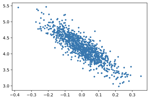
Check the distribution:

fig, ax = plt.subplots()
plt.scatter(features[:, 1], labels, s=9)
plt.show()

1.2 Reading the Dataset

Recall that training models consists of making multiple passes over the dataset, grabbing one minibatch of examples at a time, and using them to update our model.

It is worth defining a utility function to shuffle the dataset and access it in minibatches.

In the following code, we define the data_iter function to demonstrate one possible implementation of this functionality:

def data_iter(batch_size, features, labels):
    num_examples = len(features)
    indices = list(range(num_examples))
    random.shuffle(indices)

    for i in range(0, num_examples, batch_size):
        batch_indices = torch.tensor(indices[i:min(i+batch_size, num_examples)])
        yield features[batch_indices], labels[batch_indices]

Read and print the first small batch of data examples:

batch_size = 10
for X, y in data_iter(batch_size, features, labels):
    print("X: ", X)
    print("y: ", y)
    break

X:  tensor([[-0.0182,  0.1969],
        [ 0.0065,  0.0492],
        [-0.0292, -0.0455],
        [-0.2098,  0.0635],
        [-0.0983, -0.1226],
        [-0.0058,  0.0441],
        [-0.1079,  0.0113],
        [-0.0484,  0.0152],
        [ 0.1643, -0.0053],
        [-0.0322, -0.0597]])
y:  tensor([[3.4963],
        [4.0652],
        [4.2881],
        [3.5600],
        [4.4177],
        [4.0283],
        [3.9305],
        [4.0480],
        [4.5413],
        [4.3580]])

1.3 Initializing Model Parameters

Before we can begin optimizing our model’s parameters by minibatch stochastic gradient descent, we need to have some parameters in the first place.

In the following code, we initialize weights by sampling random numbers from a normal distribution with mean 0 and a standard deviation of 0.01, and setting the bias to 0:

w = torch.normal(mean=0, std=0.1, size=(2, 1), requires_grad=True)
b = torch.zeros(1, requires_grad=True)

After initializing parameters, next task is to update them until they fit our data sufficiently well.

Each update requires taking the gradient of our loss function with respect to the parameters.

Given this gradient, we can update each parameter in the direction that may reduce the loss.

1.4 Defining the Model

Define our model, relating its inputs and parameters to its outputs:

def linreg(X, w, b):
    """The linear regression model."""
    return torch.matmul(X, w)+b

1.5 Defining the Loss Function

Use squared loss function to define the loss function:

def squared_loss(y_hat, y):
    """Squared loss."""
    return (y_hat - y.reshape(y_hat.shape)) ** 2 / 2

1.6 Defining the Optimization Algorithm

Example of minibatch stochastic gradient descent:
(1) At each step, using one minibatch randomly drawn from our dataset, we will estimate the gradient of the loss with respect to our parameters.
(2) Next, we will update our parameters in the direction that may reduce the loss.

The following code applies the minibatch stochastic gradient descent update:

def sgd(params, lr, batch_size):
    # disabled gradient calculation
    with torch.no_grad():
        for param in params:
            param -= lr * param.grad / batch_size
            # clears old gradient from the last step
            param.grad.zero_()

The size of the update step is determined by the learning rate lr.

Because our loss is calculated as a sum over the minibatch of examples, we normalize our step size by the batch size (batch_size), so that the magnitude of a typical step size does not depend heavily on our choice of the batch size.

1.7 Training

In each iteration, we will grab a minibatch of training examples, and pass them through our model to obtain a set of predictions.

After calculating the loss, we initiate the backwards pass through the network, storing the gradients with respect to each parameter.

Finally, we will call the optimization algorithm sgd to update the model parameters.

In each epoch, we will iterate through the entire dataset (using the data_iter function) once passing through every example in the training dataset (assuming that the number of examples is divisible by the batch size).

The number of epochs num_epochs and the learning rate lr are both hyperparameters, which we set here to 3 and 0.03, respectively:

lr = 0.03
num_epochs = 3
net = linreg
loss = squared_loss

for epoch in range(num_epochs):
    for X, y in data_iter(batch_size, features, labels):
        l = loss(net(X, w, b), y)
        l.sum().backward()
        sgd([w, b], lr, batch_size)
    with torch.no_grad():
        train_l = loss(net(features, w, b), labels)
        print("epoch %d, loss %.4f" % (epoch, train_l.mean()))

epoch 0, loss 0.0574
epoch 1, loss 0.0541
epoch 2, loss 0.0510

References

Linear Neural Networks – Linear Regression Implementation from Scratch