R语言可视化---图形着色

library(gcookbook) # For the data set
library(tidyverse)
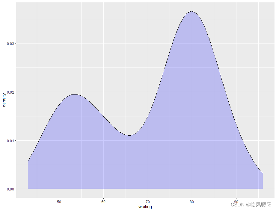
ggplot(faithful, aes(x=waiting)) +
  geom_line(stat="density") +geom_density(fill="blue", alpha=.2) 

library(gcookbook) # For the data set
library(tidyverse)
x = rnorm(n = 500, mean = 0.5, sd = 0.3)
y = rnorm(n = 500, mean = 6, sd = 1)
data = merge(x, y, by = "row.names", all = TRUE)

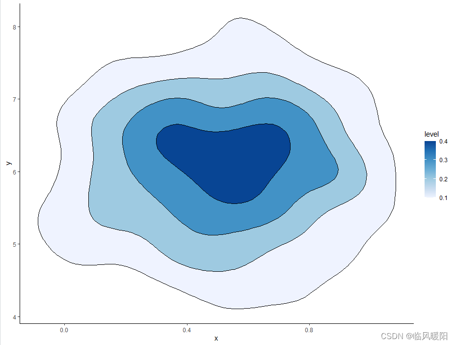
data %>% ggplot(aes(x, y))+
  stat_density_2d(geom = "polygon", contour = TRUE,
                  aes(fill = after_stat(level)), colour = "black",
                  bins = 5) +
  scale_fill_distiller(palette = "Blues", direction = 1) +
  theme_classic()

library(tidyverse)

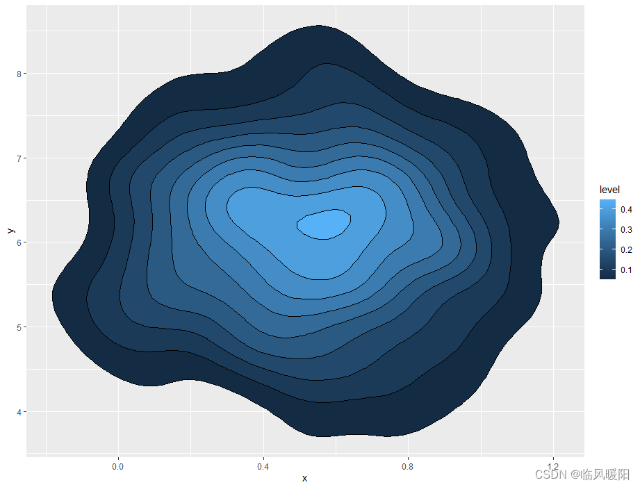
ggplot(data, aes(x=x, y=y) ) +
  stat_density_2d(aes(fill = ..level..), geom = "polygon", colour="black")

data %>% ggplot(aes(x, y))+
  stat_density_2d(geom = "polygon", contour = TRUE,
                  aes(fill = after_stat(level)), colour = "black",
                  bins = 5) +
  scale_fill_distiller(palette = "Set1", direction = 1) +
  theme_classic()

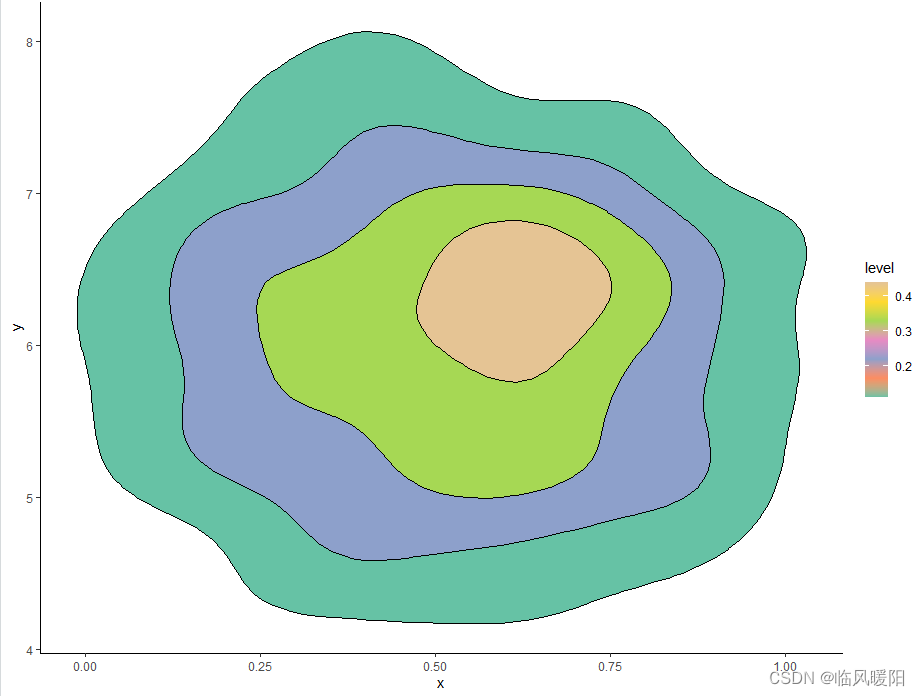
data %>% ggplot(aes(x, y))+
  stat_density_2d(geom = "polygon", contour = TRUE,
                  aes(fill = after_stat(level)), colour = "black",
                  bins = 5) +
  scale_fill_distiller(palette = "Set2", direction = 1) +
  theme_classic()

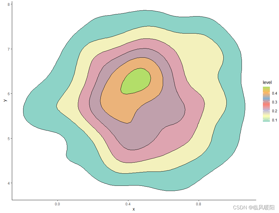
data %>% ggplot(aes(x, y))+
  stat_density_2d(geom = "polygon", contour = TRUE,
                  aes(fill = after_stat(level)), colour = "black",
                  bins = 7) +
  scale_fill_distiller(palette = "Set3", direction = 2) +
  theme_classic()

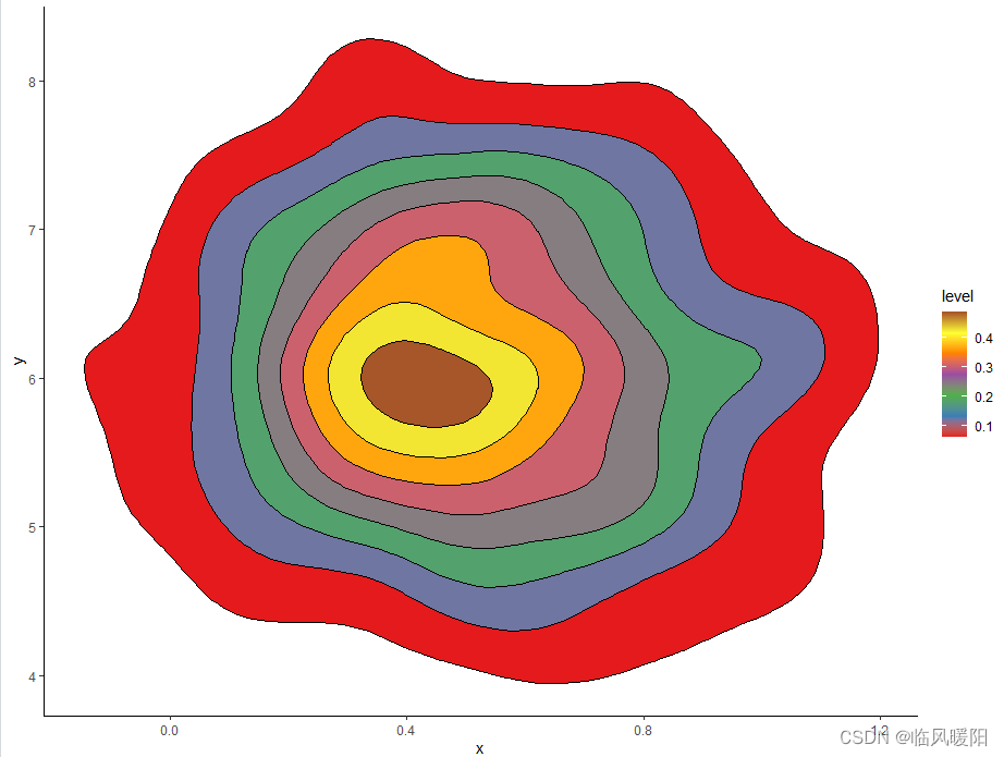
data %>% ggplot(aes(x, y))+
  stat_density_2d(geom = "polygon", contour = TRUE,
                  aes(fill = after_stat(level)), colour = "black",
                  bins = 9) +
  scale_fill_distiller(palette = "Set1", direction = 2) +
  theme_classic()

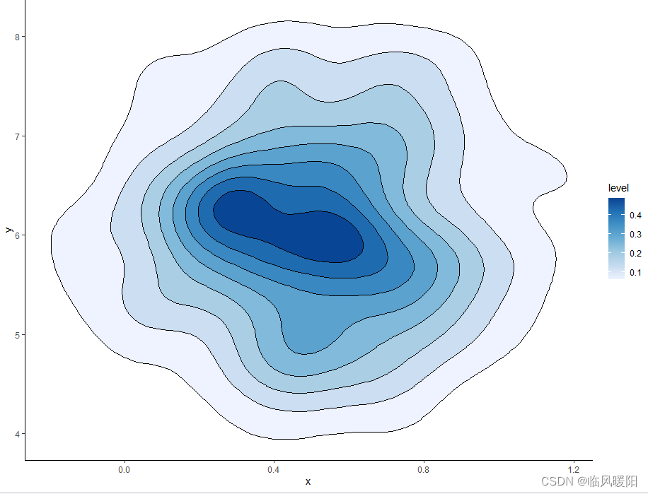
data %>% ggplot(aes(x, y))+
  stat_density_2d(geom = "polygon", contour = TRUE,
                  aes(fill = after_stat(level)), colour = "black",
                  bins = 9) +
  scale_fill_distiller(palette = "Blues", direction = 2) +
  theme_classic()

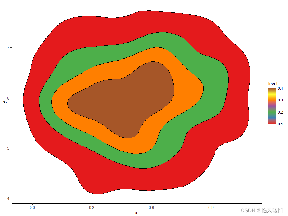
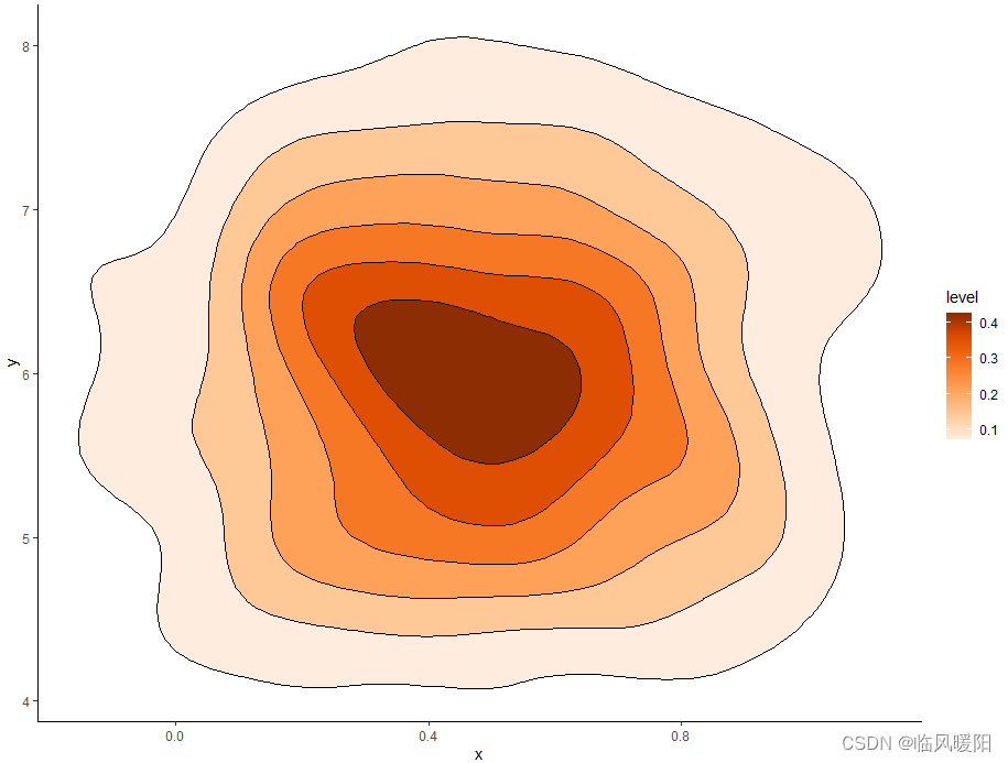
data %>% ggplot(aes(x, y))+
  stat_density_2d(geom = "polygon", contour = TRUE,
                  aes(fill = after_stat(level)), colour = "black",
                  bins = 7) +
  scale_fill_distiller(palette = "Oranges", direction = 2) +
  theme_classic()

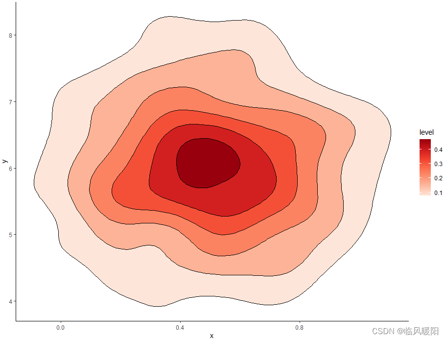
data %>% ggplot(aes(x, y))+
  stat_density_2d(geom = "polygon", contour = TRUE,
                  aes(fill = after_stat(level)), colour = "black",
                  bins = 7) +
  scale_fill_distiller(palette = "Reds", direction = 2) +
  theme_classic()

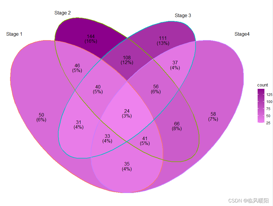
library("ggVennDiagram")
library("ggVennDiagram")
set.seed(20190708)
genes <- paste("gene",1:1000,sep="")
x <- list(
  A = sample(genes,300), 
  B = sample(genes,525), 
  C = sample(genes,440),
  D = sample(genes,350)
)
ggVennDiagram(
  x, label_alpha = 0,
  category.names = c("Stage 1","Stage 2","Stage 3", "Stage4")
) +
  ggplot2::scale_fill_gradient(low="violet",high = "darkmagenta")

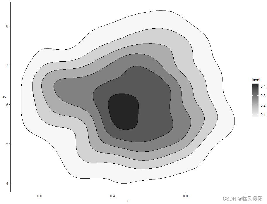
data %>% ggplot(aes(x, y))+
  stat_density_2d(geom = "polygon", contour = TRUE,
                  aes(fill = after_stat(level)), colour = "black",
                  bins = 7) +
  scale_fill_distiller(palette = "Greys", direction = 2) +
  theme_classic()
  

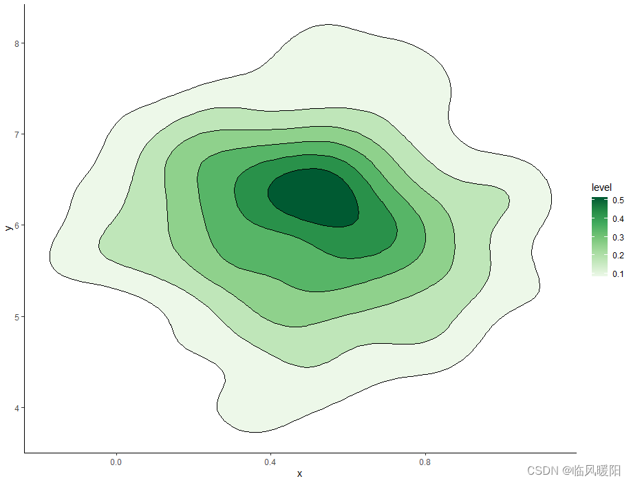
da

ta %>% ggplot(aes(x, y))+
  stat_density_2d(geom = "polygon", contour = TRUE,
                  aes(fill = after_stat(level)), colour = "black",
                  bins = 7) +
  scale_fill_distiller(palette = "Greens", direction = 2) +
  theme_classic()

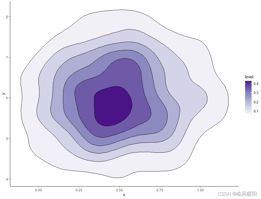
data %>% ggplot(aes(x, y))+
  stat_density_2d(geom = "polygon", contour = TRUE,
                  aes(fill = after_stat(level)), colour = "black",
                  bins = 7) +
  scale_fill_distiller(palette = "Purples", direction = 2) +
  theme_classic()

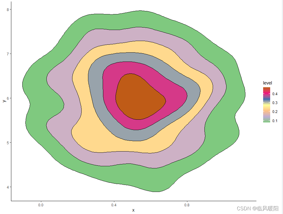
data %>% ggplot(aes(x, y))+
  stat_density_2d(geom = "polygon", contour = TRUE,
                  aes(fill = after_stat(level)), colour = "black",
                  bins = 7) +
  scale_fill_distiller(palette = "Accent", direction = 2) +
  theme_classic()

参考文献：
https://stackoom.com/question/4GtQD
https://www.docin.com/p-2219093050.html
Practical Receipes for Visualizing Data----R Graphics Cookbook —Winston Chang O’REILLY

百度文库—颜色大全：含中英文对照及色值

开发环境：RStudio和微信截屏工具