数据可视化基础与应用-04-seaborn库从入门到精通01-02

总结

本系列是数据可视化基础与应用的第04篇seaborn，是seaborn从入门到精通系列第1-2篇。本系列的目的是可以完整的完成seaborn从入门到精通。主要介绍基于seaborn实现数据可视化。

参考

参考:数据可视化-seaborn

数据集介绍

tips数据集

import seaborn as sns#seaborn图形进行数据分析
df=sns.load_dataset('tips')
df.head()#显示前五行
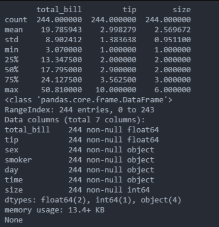
'''结果：
 	total_bill 	tip 	sex 	smoker 	day 	time 	size
0 	16.99 	  1.01  	Female 	   No 	Sun 	Dinner 	 2
1 	10.34 	  1.66 	    Male 	   No 	Sun 	Dinner 	 3
2 	21.01 	  3.50  	Male 	   No 	Sun 	Dinner 	 3
3 	23.68 	  3.31  	Male 	   No 	Sun 	Dinner 	 2
4 	24.59 	  3.61 	    Female 	   No 	Sun 	Dinner 	 4
'''

penguins数据集

penguins = sns.load_dataset(name="penguins")

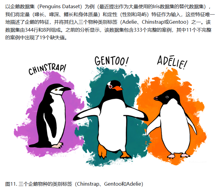
Chinstrap帽带企鹅颏带颊带帽带
Gentoo巴布亚巴布亚企鹅
Adelie阿德烈企鹅

seaborn从入门到精通01-seaborn介绍与load_dataset(“tips“)出现超时解决方案

参考

seaborn官方
seaborn官方介绍
seaborn可视化入门
【宝藏级】全网最全的Seaborn详细教程-数据分析必备手册（2万字总结）
Seaborn常见绘图总结

总结

本文主要是seaborn从入门到精通系列第1篇，本文介绍了seaborn的官方简介，同时介绍了较好的参考文档置于博客前面，读者可以重点查看参考链接。本系列的目的是可以完整的完成seaborn从入门到精通。重点参考连接

seaborn介绍

官方介绍

Seaborn is a library for making statistical graphics in Python. It builds on top of matplotlib and integrates closely with pandas data structures.
Seaborn是一个用Python制作统计图形的库。它构建在matplotlib之上，并与pandas数据结构紧密集成。

Seaborn helps you explore and understand your data. Its plotting functions operate on dataframes and arrays containing whole datasets and internally perform the necessary semantic mapping and statistical aggregation to produce informative plots. Its dataset-oriented, declarative API lets you focus on what the different elements of your plots mean, rather than on the details of how to draw them.
Seaborn帮助您探索和理解您的数据。它的绘图功能对包含整个数据集的数据框架和数组进行操作，并在内部执行必要的语义映射和统计聚合以生成信息丰富的绘图。它的面向数据集的声明性API让您可以专注于图表的不同元素的含义，而不是如何绘制它们的细节。

seaborn入门流程

# Import seaborn
import seaborn as sns

# Apply the default theme
sns.set_theme()

# Load an example dataset 需要
# tips = sns.load_dataset("tips")
tips = sns.load_dataset("tips",cache=True,data_home=r'.\seaborn-data')

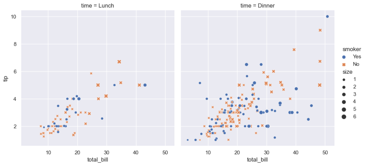
# Create a visualization
sns.relplot(
    data=tips,
    x="total_bill", y="tip", col="time",
    hue="smoker", style="smoker", size="size",
)

如果加载数据时出现问题，可以参考博客
seaborn从入门到精通-seaborn在load_dataset(“tips“)出现超时的错误

# Import seaborn
import seaborn as sns

Seaborn is the only library we need to import for this simple example. By convention, it is imported with the shorthand sns.
对于这个简单的示例，我们需要导入的库只有Seaborn。按照惯例，它与简写sns一起导入。
Behind the scenes, seaborn uses matplotlib to draw its plots. For interactive work, it’s recommended to use a Jupyter/IPython interface in matplotlib mode, or else you’ll have to call matplotlib.pyplot.show() when you want to see the plot.
在幕后，seaborn使用matplotlib绘制它的情节。对于交互式工作，建议在matplotlib模式下使用Jupyter/IPython接口，否则当您想要查看绘图时，必须调用matplotlib.pyplot.show()。

# Apply the default theme
sns.set_theme()

This uses the matplotlib rcParam system and will affect how all matplotlib plots look, even if you don’t make them with seaborn. Beyond the default theme, there are several other options, and you can independently control the style and scaling of the plot to quickly translate your work between presentation contexts (e.g., making a version of your figure that will have readable fonts when projected during a talk). If you like the matplotlib defaults or prefer a different theme, you can skip this step and still use the seaborn plotting functions.
这将使用matplotlib rcParam系统，并将影响所有matplotlib图的外观，即使您没有使用seaborn创建它们。除了默认主题之外，还有其他几个选项，您可以独立控制图形的样式和缩放，以便在不同的演示上下文之间快速转换您的工作(例如，制作一个在演讲期间投影时具有可读字体的图形版本)。如果您喜欢matplotlib默认值或喜欢不同的主题，您可以跳过此步骤，仍然使用seaborn绘图函数。

# Load an example dataset
#tips = sns.load_dataset("tips")
tips = sns.load_dataset("tips",cache=True,data_home=r'.\seaborn-data')

Most code in the docs will use the load_dataset() function to get quick access to an example dataset. There’s nothing special about these datasets: they are just pandas dataframes, and we could have loaded them with pandas.read_csv() or built them by hand. Most of the examples in the documentation will specify data using pandas dataframes, but seaborn is very flexible about the data structures that it accepts.
文档中的大多数代码将使用load_dataset()函数来快速访问示例数据集。这些数据集没有什么特别之处:它们只是pandas数据框架，我们可以用pandas.read_csv()加载它们，也可以手工构建它们。文档中的大多数示例都将使用pandas数据框架指定数据，但是seaborn对于它所接受的数据结构非常灵活。

# Create a visualization
sns.relplot(
    data=tips,
    x="total_bill", y="tip", col="time",
    hue="smoker", style="smoker", size="size",
)

This plot shows the relationship between five variables in the tips dataset using a single call to the seaborn function relplot().
这个图通过对seaborn函数relplot()的一次调用显示了tips数据集中五个变量之间的关系。
Notice how we provided only the names of the variables and their roles in the plot. Unlike when using matplotlib directly, it wasn’t necessary to specify attributes of the plot elements in terms of the color values or marker codes.
请注意，我们如何仅提供变量的名称及其在图中的角色。与直接使用matplotlib不同，不需要根据颜色值或标记代码指定绘图元素的属性。
Behind the scenes, seaborn handled the translation from values in the dataframe to arguments that matplotlib understands. This declarative approach lets you stay focused on the questions that you want to answer, rather than on the details of how to control matplotlib.
在幕后，seaborn处理从数据框架中的值到matplotlib能够理解的参数的转换。这种声明性方法使您能够将注意力集中在想要回答的问题上，而不是集中在如何控制matplotlib的细节上。

sns.load_dataset(“tips”)出现超时的错误

# Import seaborn
import seaborn as sns

# Apply the default theme
sns.set_theme()

# Load an example dataset 需要
# tips = sns.load_dataset("tips")
tips = sns.load_dataset("tips",cache=True,data_home=r'.\seaborn-data')

# Create a visualization
sns.relplot(
    data=tips,
    x="total_bill", y="tip", col="time",
    hue="smoker", style="smoker", size="size",
)

以上代码往往出现连接超时的错误

TimeoutError: [WinError 10060] 由于连接方在一段时间后没有正确答复或连接的主机没有反应，连接尝试失败。

下载seaborn-data数据

这是因为seaborn需要从网络或是tips数据集，这里提供一个码云的下载连接，下载后，把数据集解压到本地。

方法一：seaborn-data数据到默认位置

进入python交互界面，输入

import seaborn as sns
sns.utils.get_data_home()

返回seaborn的默认读取文件的地址

‘C:\Users\DELL\AppData\Local\seaborn\seaborn\Cache’

把解压后的seaborn-data-master目录中的所有文件

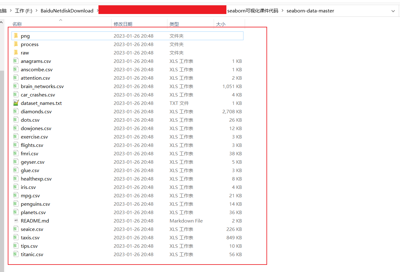
拷贝到seaborn-data目录下

‘C:\Users\DELL\AppData\Local\seaborn\seaborn\Cache’

方法二：通过指定data_home确定文件位置

解压后的seaborn-data-master目录中的所有文件放在工程目录的seaborn-data目录下，或是放在d盘的seaborn目录下。
然后通过load_dataset时指定data_home完成文件读取。

tips = sns.load_dataset("tips",cache=True,data_home=r'.\seaborn-data')
#tips = sns.load_dataset("tips",cache=True,data_home=r'd:\seaborn-data')

采用以上两种方法后，都可以解决出现加载数据失败的问题

seaborn从入门到精通02-绘图功能概述

总结

本文主要是seaborn从入门到精通系列第2篇，本文介绍了seaborn的绘图功能，包括Figure-level和axes-level级别的使用方法，以及组合数据绘图函数，同时介绍了较好的参考文档置于博客前面，读者可以重点查看参考链接。本系列的目的是可以完整的完成seaborn从入门到精通。重点参考连接

参考

seaborn官方
seaborn官方介绍
seaborn可视化入门
【宝藏级】全网最全的Seaborn详细教程-数据分析必备手册（2万字总结）
Seaborn常见绘图总结

A high-level API for statistical graphics 用于统计图形的高级API

There is no universally best way to visualize data. Different questions are best answered by different plots. Seaborn makes it easy to switch between different visual representations by using a consistent dataset-oriented API.
没有普遍的最佳方法来可视化数据。不同的问题最好由不同的情节来回答。通过使用一致的面向数据集的API, Seaborn可以轻松地在不同的可视化表示之间切换。

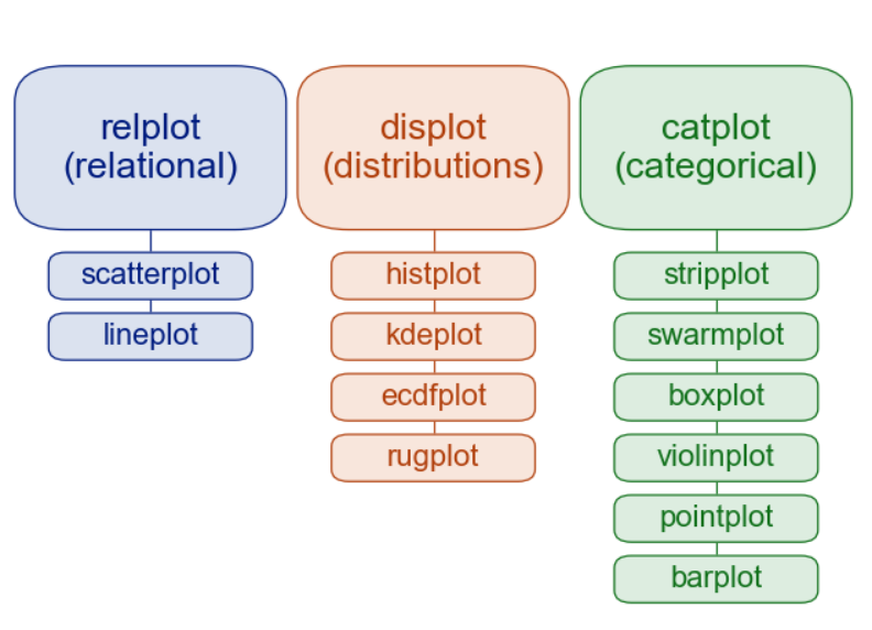
Similar functions for similar tasks

seaborn命名空间是扁平的;所有的功能都可以在顶层访问。但是代码本身是层次结构的，函数模块通过不同的方式实现类似的可视化目标。大多数文档都是围绕这些模块构建的:

relational “关系型”
distributional “分布型”
categorical “分类型”

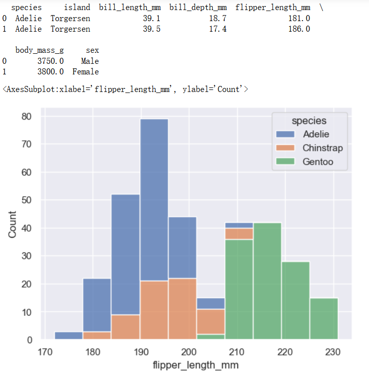
distributional模块下的histplot

penguins = sns.load_dataset("penguins",cache=True,data_home=r'.\seaborn-data')
print(penguins[0:5])
sns.histplot(data=penguins, x="flipper_length_mm", hue="species", multiple="stack")

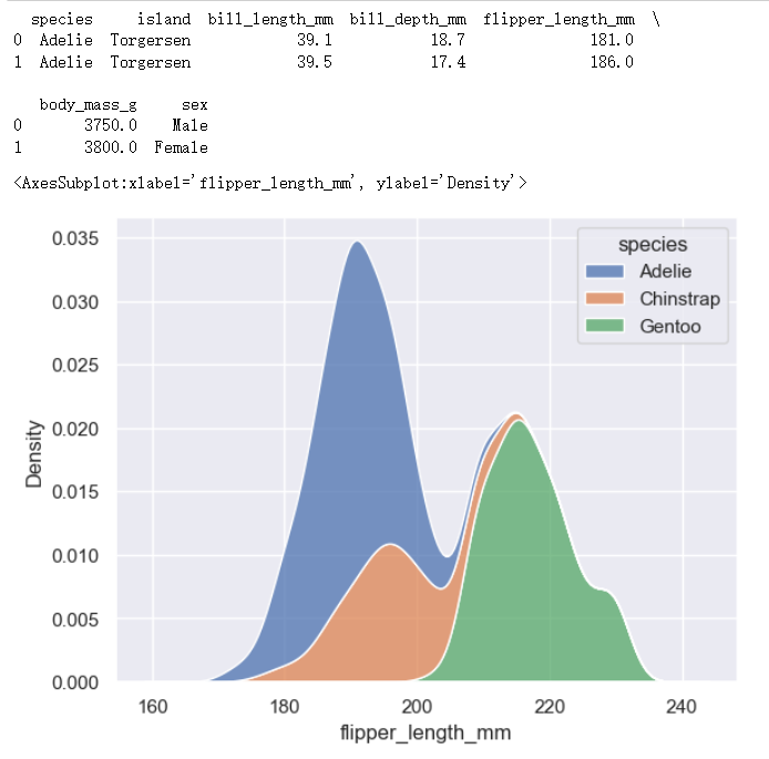
distributional模块下的kdeplot

Along with similar, but perhaps less familiar, options such as kernel density estimation:
还有类似的，但可能不太熟悉的选项，如核密度估计

penguins = sns.load_dataset("penguins",cache=True,data_home=r'.\seaborn-data')
print(penguins[0:2])
sns.kdeplot(data=penguins, x="flipper_length_mm", hue="species", multiple="stack")

统一模块中的函数共享大量底层代码，并提供类似的功能，而这些功能在库的其他组件中可能不存在(例如上面示例中的multiple=“stack”)。

Figure-level vs. axes-level functions

In addition to the different modules, there is a cross-cutting classification of seaborn functions as “axes-level” or “figure-level”. The examples above are axes-level functions. They plot data onto a single matplotlib.pyplot.Axes object, which is the return value of the function.
除了不同的模块外，还将seaborn函数交叉分类为“axes-level轴级”或“figure-level图形级”。上面的例子（histplot和kdeplot）是轴级函数。它们将数据绘制到单个matplotlib.pyplot.Axes对象上，该对象是函数的返回值。
In contrast, figure-level functions interface with matplotlib through a seaborn object, usually a FacetGrid, that manages the figure. Each module has a single figure-level function, which offers a unitary interface to its various axes-level functions. The organization looks a bit like this:
相比之下，图形级函数通过管理图形的seaborn对象(通常是FacetGrid)与matplotlib进行接口。每个模块都有一个唯一的一个figure-level functions，为其各种axes-level functions提供了一个统一的接口。该组织看起来有点像这样:

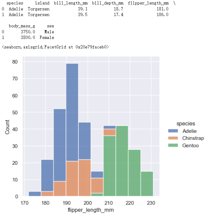
distributional模块下的displot()绘制histplot图

例如，displot()是分布模块的图形级函数。它的默认行为是绘制直方图，在幕后使用与histplot()相同的代码:

penguins = sns.load_dataset("penguins",cache=True,data_home=r'.\seaborn-data')
print(penguins[0:2])
# sns.histplot(data=penguins, x="flipper_length_mm", hue="species", multiple="stack")
# sns.kdeplot(data=penguins, x="flipper_length_mm", hue="species", multiple="stack")
sns.displot(data=penguins, x="flipper_length_mm", hue="species", multiple="stack")

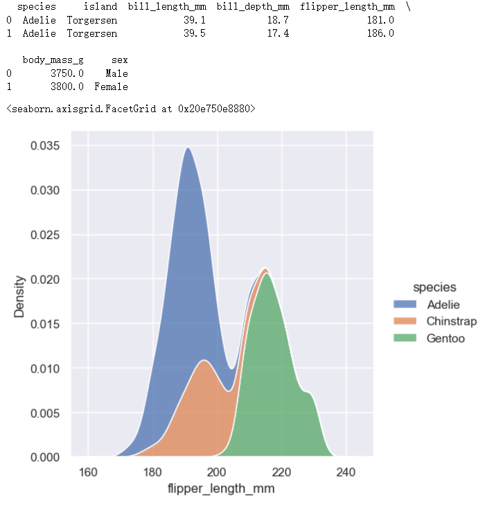
distributional模块下的displot()绘制kdetplot图

To draw a kernel density plot instead, using the same code as kdeplot(), select it using the kind parameter:
要绘制内核密度图，使用与kdeploy()相同的代码，使用kind参数选择它:

penguins = sns.load_dataset("penguins",cache=True,data_home=r'.\seaborn-data')
print(penguins[0:2])
# sns.histplot(data=penguins, x="flipper_length_mm", hue="species", multiple="stack")
# sns.kdeplot(data=penguins, x="flipper_length_mm", hue="species", multiple="stack")
# sns.displot(data=penguins, x="flipper_length_mm", hue="species", multiple="stack")
sns.displot(data=penguins, x="flipper_length_mm", hue="species", multiple="stack", kind="kde")

distributional模块下的Figure和axes级别的绘图对比-内核密度图

penguins = sns.load_dataset("penguins",cache=True,data_home=r'.\seaborn-data')
print(penguins[0:2])
# sns.histplot(data=penguins, x="flipper_length_mm", hue="species", multiple="stack")
sns.kdeplot(data=penguins, x="flipper_length_mm", hue="species", multiple="stack")
# sns.displot(data=penguins, x="flipper_length_mm", hue="species", multiple="stack")
sns.displot(data=penguins, x="flipper_length_mm", hue="species", multiple="stack", kind="kde")

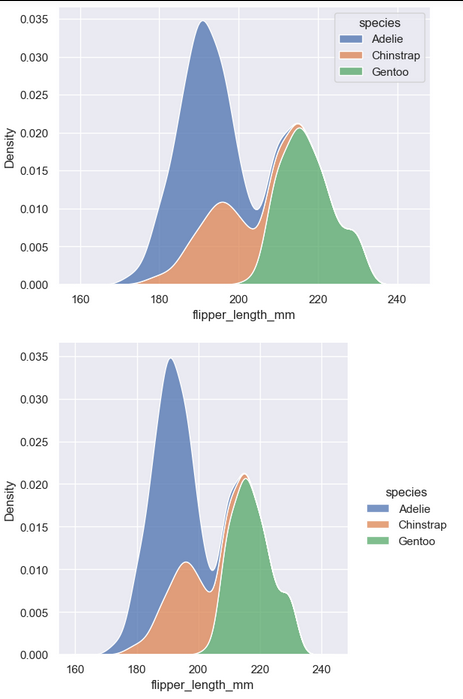
You’ll notice that the figure-level plots look mostly like their axes-level counterparts, but there are a few differences. Notably, the legend is placed outside the plot. They also have a slightly different shape (more on that shortly).
您将注意到，图形级的图与它们的轴级对应图非常相似，但也有一些不同之处。值得注意的是，传说被放置在情节之外。它们的形状也略有不同(稍后会详细介绍)。
The most useful feature offered by the figure-level functions is that they can easily create figures with multiple subplots. For example, instead of stacking the three distributions for each species of penguins in the same axes, we can “facet” them by plotting each distribution across the columns of the figure:
figure-level functions 提供的最有用的特性是，figure-level functions 可以轻松地创建具有多个子图的图形。例如，我们不需要将每种企鹅的三个分布叠加在同一个轴上，而是可以通过在图的列上绘制每个分布来“面化”它们:
penguins = sns.load_dataset(“penguins”,cache=True,data_home=r’.\seaborn-data’)
sns.displot(data=penguins, x=“flipper_length_mm”, hue=“species”, col=“species”

The figure-level functions wrap their axes-level counterparts and pass the kind-specific keyword arguments (such as the bin size for a histogram) down to the underlying function. That means they are no less flexible, but there is a downside: the kind-specific parameters don’t appear in the function signature or docstrings. Some of their features might be less discoverable, and you may need to look at two different pages of the documentation before understanding how to achieve a specific goal.
figure-level functions 包装它们的axes-level对应对象，并将特定于种类的关键字参数(例如直方图的bin大小)传递给底层函数。这意味着它们同样灵活，但也有一个缺点:特定于种类的参数不会出现在函数签名或文档字符串中。它们的一些特性可能不太容易发现，在理解如何实现特定目标之前，您可能需要查看两个不同的文档页面。

Axes-level functions make self-contained plots 轴级函数制作自包含的图

The axes-level functions are written to act like drop-in replacements for matplotlib functions. While they add axis labels and legends automatically, they don’t modify anything beyond the axes that they are drawn into. That means they can be composed into arbitrarily-complex matplotlib figures with predictable results.
The axes-level functions call matplotlib.pyplot.gca() internally, which hooks into the matplotlib state-machine interface so that they draw their plots on the “currently-active” axes. But they additionally accept an ax= argument, which integrates with the object-oriented interface and lets you specify exactly where each plot should go:

penguins = sns.load_dataset("penguins",cache=True,data_home=r'.\seaborn-data')
print(penguins[0:2])
"""
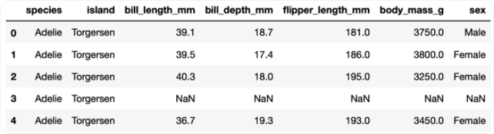
  species     island  bill_length_mm  bill_depth_mm  flipper_length_mm  \
0  Adelie  Torgersen            39.1           18.7              181.0   
1  Adelie  Torgersen            39.5           17.4              186.0   

   body_mass_g     sex  
0       3750.0    Male  
1       3800.0  Female  

"""
f, axs = plt.subplots(1, 2, figsize=(8, 4), gridspec_kw=dict(width_ratios=[4, 3]))
sns.scatterplot(data=penguins, x="flipper_length_mm", y="bill_length_mm", hue="species", ax=axs[0])
sns.histplot(data=penguins, x="species", hue="species", shrink=.8, alpha=.8, legend=False, ax=axs[1])
f.tight_layout()

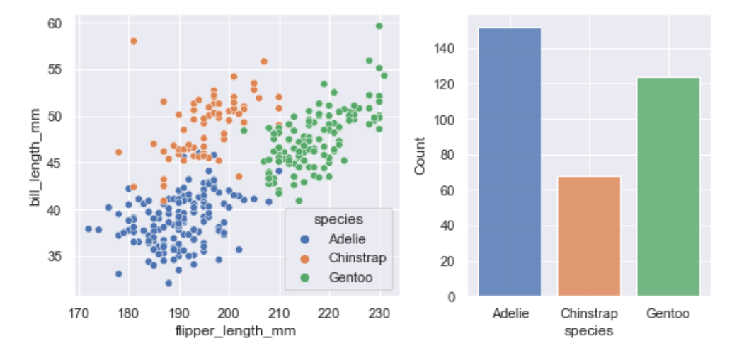
Figure-level functions own their figure 图形级函数拥有它们的图形

In contrast, figure-level functions cannot (easily) be composed with other plots. By design, they “own” their own figure, including its initialization, so there’s no notion of using a figure-level function to draw a plot onto an existing axes. This constraint allows the figure-level functions to implement features such as putting the legend outside of the plot.
相比之下，图形级函数不能(轻易地)与其他图组合。按照设计，它们“拥有”自己的图形，包括其初始化，因此不存在使用图形级函数在现有轴上绘制图形的概念。这个约束允许图形级函数实现一些特性，比如将图例放在图之外。
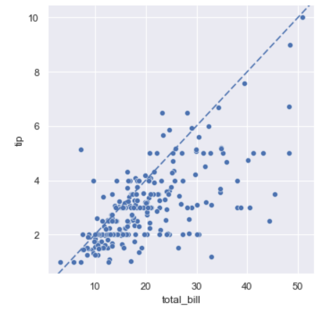
Nevertheless, it is possible to go beyond what the figure-level functions offer by accessing the matplotlib axes on the object that they return and adding other elements to the plot that way:
然而，通过访问返回对象上的matplotlib轴，并以这种方式将其他元素添加到图中，可以超越图形级函数所提供的功能:

tips = sns.load_dataset("tips",cache=True,data_home=r'.\seaborn-data')
print(tips[0:2])
"""
   total_bill   tip     sex smoker  day    time  size
0       16.99  1.01  Female     No  Sun  Dinner     2
1       10.34  1.66    Male     No  Sun  Dinner     3
"""
g = sns.relplot(data=tips, x="total_bill", y="tip")
g.ax.axline(xy1=(10, 2), slope=.2, color="b", dashes=(5, 2))

Customizing plots from a figure-level function 定制图形级函数的图形

The figure-level functions return a FacetGrid instance, which has a few methods for customizing attributes of the plot in a way that is “smart” about the subplot organization. For example, you can change the labels on the external axes using a single line of code:
图级函数返回一个FacetGrid实例，该实例具有一些方法，用于以一种关于子图组织的“智能”方式定制图的属性。例如，您可以使用一行代码更改外部轴上的标签:

g = sns.relplot(data=penguins, x="flipper_length_mm", y="bill_length_mm", col="sex")
g.set_axis_labels("Flipper length (mm)", "Bill length (mm)")

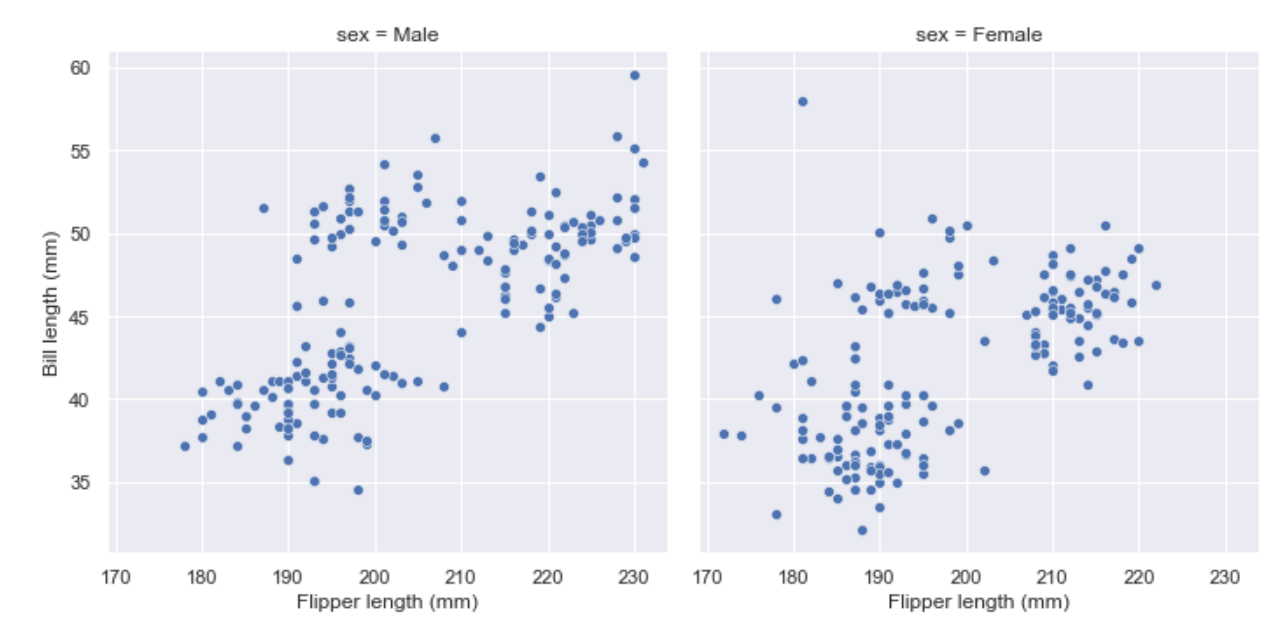
While convenient, this does add a bit of extra complexity, as you need to remember that this method is not part of the matplotlib API and exists only when using a figure-level function.
虽然方便，但这确实增加了一些额外的复杂性，因为您需要记住，此方法不是matplotlib API的一部分，仅在使用图形级函数时存在。

Specifying figure sizes 指定图形大小

To increase or decrease the size of a matplotlib plot, you set the width and height of the entire figure, either in the global rcParams, while setting up the plot (e.g. with the figsize parameter of matplotlib.pyplot.subplots()), or by calling a method on the figure object (e.g. matplotlib.Figure.set_size_inches()). When using an axes-level function in seaborn, the same rules apply: the size of the plot is determined by the size of the figure it is part of and the axes layout in that figure.
要增加或减少matplotlib图形的大小，您可以在全局rcParams中设置整个图形的宽度和高度，同时设置图形(例如使用matplotlib.pyplot.subplots()的figsize参数)，或者通过调用图形对象上的方法(例如matplotlib. figure . set_size_吋())。当在seaborn中使用轴级函数时，同样的规则也适用:图的大小由它所在的图形的大小和该图中的轴布局决定。
When using a figure-level function, there are several key differences. First, the functions themselves have parameters to control the figure size (although these are actually parameters of the underlying FacetGrid that manages the figure). Second, these parameters, height and aspect, parameterize the size slightly differently than the width, height parameterization in matplotlib (using the seaborn parameters, width = height * aspect). Most importantly, the parameters correspond to the size of each subplot, rather than the size of the overall figure.
在使用图形级函数时，有几个关键的区别。首先，函数本身具有控制图形大小的参数(尽管这些实际上是管理图形的底层FacetGrid的参数)。其次，这些参数，高度和方面，在matplotlib中参数化的大小与宽度、高度略有不同(使用seaborn参数，宽度=高度*方面)。最重要的是，这些参数对应于每个子图的大小，而不是整个图形的大小。
To illustrate the difference between these approaches, here is the default output of matplotlib.pyplot.subplots() with one subplot:

为了说明这些方法之间的区别，下面是matplotlib.pyplot.subplots()的默认输出，其中有一个子plot:
A figure with multiple columns will have the same overall size, but the axes will be squeezed horizontally to fit in the space:
有多个列的图形将具有相同的总体大小，但轴将水平压缩以适应空间:

f, ax = plt.subplots()
f, ax = plt.subplots(1, 2, sharey=True)

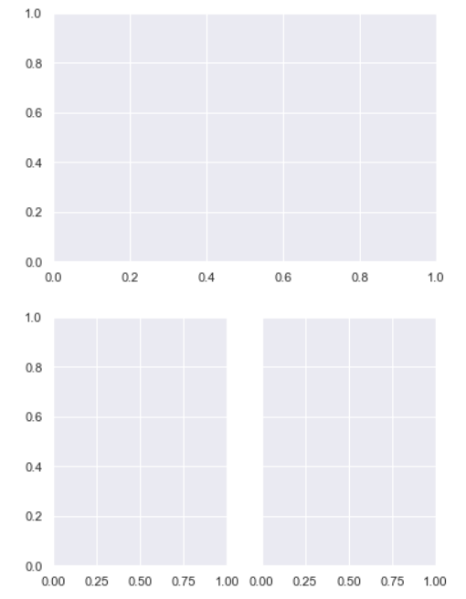
In contrast, a plot created by a figure-level function will be square. To demonstrate that, let’s set up an empty plot by using FacetGrid directly. This happens behind the scenes in functions like relplot(), displot(), or catplot():
相反，由图形级函数创建的图形将是正方形的。为了演示这一点，让我们直接使用FacetGrid来设置一个空图。这发生在relplot()， displot()或catplot()等函数的幕后:
When additional columns are added, the figure itself will become wider, so that its subplots have the same size and shape:
当添加额外的列时，图形本身将变得更宽，因此其子图具有相同的大小和形状:
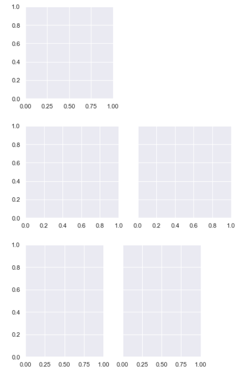
And you can adjust the size and shape of each subplot without accounting for the total number of rows and columns in the figure:
而且你可以调整每个子图的大小和形状，而不用考虑图中的行和列的总数:

g = sns.FacetGrid(penguins) # 第1行
g = sns.FacetGrid(penguins, col="sex") # 第2行
g = sns.FacetGrid(penguins, col="sex", height=3.5, aspect=.75) # 第3行

The upshot is that you can assign faceting variables without stopping to think about how you’ll need to adjust the total figure size. A downside is that, when you do want to change the figure size, you’ll need to remember that things work a bit differently than they do in matplotlib.
结果是，你可以分配面形变量，而不需要停下来考虑如何调整总图形大小。缺点是，当您确实想要更改图形大小时，您需要记住，事情的工作方式与在matplotlib中的工作方式略有不同。

Relative merits of figure-level functions 相对优点figure-level functions

Here is a summary of the pros and cons that we have discussed above:
下面是我们上面讨论过的优点和缺点的总结

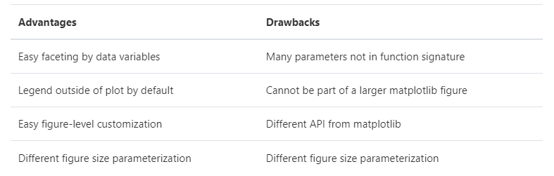
On balance, the figure-level functions add some additional complexity that can make things more confusing for beginners, but their distinct features give them additional power. The tutorial documentation mostly uses the figure-level functions, because they produce slightly cleaner plots, and we generally recommend their use for most applications. The one situation where they are not a good choice is when you need to make a complex, standalone figure that composes multiple different plot kinds. At this point, it’s recommended to set up the figure using matplotlib directly and to fill in the individual components using axes-level functions.
总的来说，图形级函数增加了一些额外的复杂性，这可能会使初学者更加困惑，但它们独特的特性赋予了它们额外的功能。教程文档主要使用图形级函数，因为它们生成的图形稍微清晰一些，我们通常建议在大多数应用程序中使用它们。当你需要制作一个复杂的、独立的、包含多种不同情节类型的人物时，它们就不是一个好的选择。此时，建议直接使用matplotlib设置图形并填充

Combining multiple views on the data 组合数据的多个视图

Two important plotting functions in seaborn don’t fit cleanly into the classification scheme discussed above. These functions, jointplot() and pairplot(), employ multiple kinds of plots from different modules to represent multiple aspects of a dataset in a single figure. Both plots are figure-level functions and create figures with multiple subplots by default. But they use different objects to manage the figure: JointGrid and PairGrid, respectively.
seaborn中两个重要的标绘函数不完全适合上面讨论的分类方案。这些函数jointplot()和pairplot()使用来自不同模块的多种图来在单个图中表示数据集的多个方面。这两个图都是图形级函数，默认情况下创建带有多个子图的图形。但是它们使用不同的对象来管理图形:分别是JointGrid和PairGrid

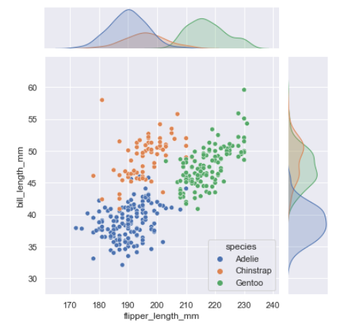
jointplot()

jointplot() plots the relationship or joint distribution of two variables while adding marginal axes that show the univariate distribution of each one separately:
Jointplot()绘制两个变量的关系或联合分布，同时添加边缘轴，分别显示每个变量的单变量分布:

# Import seaborn
import seaborn as sns
import matplotlib.pyplot as plt

# Load an example dataset 需要
# tips = sns.load_dataset("tips")
penguins = sns.load_dataset("penguins",cache=True,data_home=r'.\seaborn-data')

sns.jointplot(data=penguins, x="flipper_length_mm", y="bill_length_mm", hue="species")

Behind the scenes, these functions are using axes-level functions that you have already met (scatterplot() and kdeplot()), and they also have a kind parameter that lets you quickly swap in a different representation:
在幕后，这些函数使用的是你已经见过的轴级函数(scatterplot()和kdeploy())，它们还有一个kind参数，可以让你快速交换不同的表示形式:

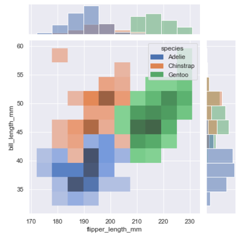
# Import seaborn
import seaborn as sns
import matplotlib.pyplot as plt

# Load an example dataset 需要
# tips = sns.load_dataset("tips")
penguins = sns.load_dataset("penguins",cache=True,data_home=r'.\seaborn-data')

# sns.jointplot(data=penguins, x="flipper_length_mm", y="bill_length_mm", hue="species")
sns.jointplot(data=penguins, x="flipper_length_mm", y="bill_length_mm", hue="species", kind="hist")

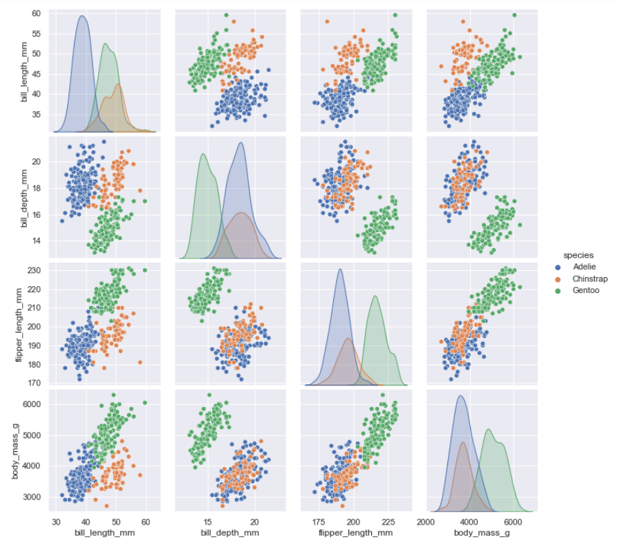
pairplot()

pairplot() is similar — it combines joint and marginal views — but rather than focusing on a single relationship, it visualizes every pairwise combination of variables simultaneously:
Pairplot()是类似的-它结合了联合视图和边缘视图-但不是专注于单个关系，它同时可视化每个变量的成对组合:

# Import seaborn
import seaborn as sns
import matplotlib.pyplot as plt

# Load an example dataset 需要
# tips = sns.load_dataset("tips")
penguins = sns.load_dataset("penguins",cache=True,data_home=r'.\seaborn-data')

# sns.jointplot(data=penguins, x="flipper_length_mm", y="bill_length_mm", hue="species")
# sns.jointplot(data=penguins, x="flipper_length_mm", y="bill_length_mm", hue="species", kind="hist")
sns.pairplot(data=penguins, hue="species")