贝叶斯优化（一）：最简单的代码篇-CSDN博客

本文链接：https://blog.csdn.net/m0_50908842/article/details/147710633

贝叶斯优化目前有完整的开源库，理解起来仍有难度

结合自己的理解对贝叶斯优化过程进行简化

1. 导入包

import numpy as np
import matplotlib.pyplot as plt

2. 函数定义

包括目标函数和高斯过程中的核函数

# 定义目标函数
def target(x):
    return np.exp(-(x - 2) ** 2) + np.exp(-(x - 6) ** 2 / 10) + 1 / (x ** 2 + 1)


# 核函数定义
def kernel(x1, x2, l=1.0, sigma_f=1.0):
    dist_matrix = np.sum(x1 ** 2, 1).reshape(-1, 1) + np.sum(x2 ** 2, 1) - 2 * np.dot(x1, x2.T)
    return sigma_f ** 2 * np.exp(-0.5 * dist_matrix / l ** 2)

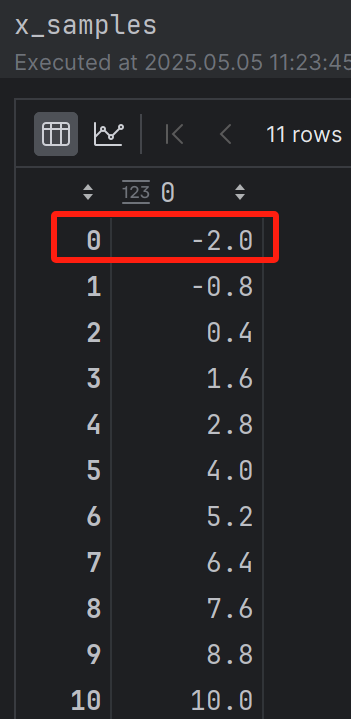
3. 生成样本点

# 生成样本点
x_samples = np.linspace(-2, 10, 11).reshape(-1, 1)
y_true = target(x_samples)

4. 高斯过程

先验没有任何点信息的时候

# 初始高斯过程先验
mu_prior = np.zeros_like(x_samples).ravel()
cov_prior = kernel(x_samples, x_samples)
std_prior = 1.96 * np.sqrt(np.diag(cov_prior))

5. 绘制图形

# 绘制先验分布
plt.figure(figsize=(10, 6))
plt.fill_between(x_samples.ravel(), mu_prior + std_prior, mu_prior - std_prior,
                 alpha=0.2, label='Prior 95% CI')
plt.plot(x_samples, y_true, 'r--', label='True Function')
plt.plot(x_samples, mu_prior, 'b-', label='Posterior Mean')
plt.title('Prior Distribution')
plt.legend()
plt.grid()
plt.show()

结果图

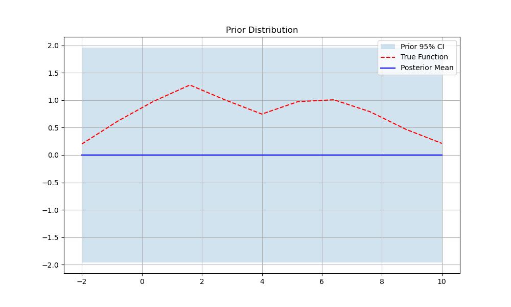
注意点：x_samples 比较粗糙，是为了更好的看过程数据

6. 加入观测点第一次

# 定义初始观测点
observations = {
    "x": np.array([-2]),  # 手工指定的初始点
    "y": target(np.array([-2]))
}


obs_x=observations["x"].reshape(-1, 1)
obs_y=observations["y"].reshape(-1, 1)

7. 后验计算

# 高斯过程后验计算
K11 = kernel(x_samples, x_samples)  # (100,100)
K22 = kernel(obs_x, obs_x)  # (n,n)
K12 = kernel(x_samples, obs_x)  # (100,n)
K21 = K12.T  # (n,100)

# 加入噪声防止奇异矩阵
K22 += 1e-6 * np.eye(len(obs_x))
K22_inv = np.linalg.inv(K22)

# 后验计算
mu_post = K12 @ K22_inv @ obs_y.reshape(-1, 1)
cov_post = K11 - K12 @ K22_inv @ K21

mu_post = mu_post.ravel()
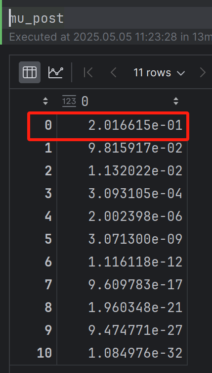
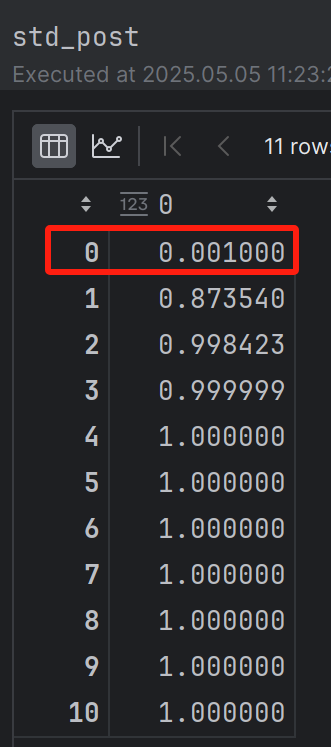
std_post = np.sqrt(np.diag(cov_post))

mu_post：观测点为-2，值为0.201662，所以mu_post对应x_samples等于-2时候的值为0.201662

std_post：为cov矩阵的对角线元素的平方，因为-2处的值已知，所以-2处的std_post最小。

对应图：

8. 后验画图

# 创建带UCB子图的画布
fig, (ax1, ax2) = plt.subplots(2, 1, figsize=(12, 10), gridspec_kw={'height_ratios': [2, 1]})
plt.ion()  # 启用交互模式
# 可视化后验分布及观测点
plt.figure(figsize=(10, 6))
# 上栏：高斯过程可视化
ax1.fill_between(x_samples.ravel(), mu_post + std_post, mu_post - std_post,
                 alpha=0.2, label='95% CI')
ax1.plot(x_samples, y_true, 'r--', label='True Function')
ax1.plot(x_samples, mu_post, 'b-', label='GP Mean')
ax1.scatter(obs_x, obs_y, c='red', s=100, marker='x', label='Observations')
ax1.set_title(f'Gaussian Process (κ={kappa})')
ax1.legend()
ax1.grid()

# 下栏：UCB可视化
ax2.plot(x_samples, ucb, 'g-', label='UCB')
ax2.scatter(x_samples[np.argmax(ucb)], np.max(ucb),
            c='gold', s=100, marker='*', edgecolors='k', label='Max UCB')
ax2.set_title('Acquisition Function (UCB)')
ax2.legend()
ax2.grid()

plt.tight_layout()
plt.pause(0.1)

结果图

9. 加入观测点第二次

采用的获得函数是ucb，ucb最大时的x值是0.4

# 选取最大UCB点作为新观测点
x_new = x_samples[np.argmax(ucb)]
y_new = target(x_new)

# 更新观测点集合
observations["x"] = np.append(observations["x"], x_new)
observations["y"] = np.append(observations["y"], y_new)

# 重新准备观测数据
obs_x = observations["x"].reshape(-1, 1)  # 现在有2个观测点
obs_y = observations["y"].reshape(-1, 1)

10. 后验计算

# 重新计算后验分布
K11 = kernel(x_samples, x_samples)  # 保持(11,11)
K22 = kernel(obs_x, obs_x)  # 现在(2,2)
K12 = kernel(x_samples, obs_x)  # (11,2)
K21 = K12.T  # (2,11)

# 添加噪声项
K22 += 1e-6 * np.eye(len(obs_x))
K22_inv = np.linalg.inv(K22)

# 后验更新
mu_post = K12 @ K22_inv @ obs_y  # (11,2) @ (2,2) @ (2,1) -> (11,1)
cov_post = K11 - K12 @ K22_inv @ K21

mu_post = mu_post.ravel()
std_post = np.sqrt(np.diag(cov_post))

11. 后验画图

# 更新可视化
ax1.cla()
ax2.cla()

# 创建带UCB子图的画布
fig, (ax1, ax2) = plt.subplots(2, 1, figsize=(12, 10), gridspec_kw={'height_ratios': [2, 1]})
plt.ion()  # 启用交互模式
# 可视化后验分布及观测点
plt.figure(figsize=(10, 6))
# 上栏更新
ax1.fill_between(x_samples.ravel(), mu_post + std_post, mu_post - std_post,
                 alpha=0.2, label='95% CI')
ax1.plot(x_samples, y_true, 'r--', label='True Function')
ax1.plot(x_samples, mu_post, 'b-', label='GP Mean')
ax1.scatter(obs_x, obs_y, c='red', s=100, marker='x', label='Observations')
ax1.set_title(f'Gaussian Process (κ={kappa}) - Iteration 2')
ax1.grid()

# 下栏更新
ax2.plot(x_samples, ucb, 'g-', label='UCB')
ax2.scatter(x_samples[np.argmax(ucb)], np.max(ucb),
            c='gold', s=100, marker='*', edgecolors='k', label='Max UCB')
ax2.set_title('Acquisition Function (UCB) - Updated')
ax2.grid()
plt.tight_layout()
plt.pause(0.1)

结果图