【Machine Learning】4.特征缩放和学习率

本节主要介绍如何处理多个特征，以及怎么调整多元线性回归时的学习率 $\alpha$

1.导入

1.1 导入包

import numpy as np
np.set_printoptions(precision=2)
import matplotlib.pyplot as plt
dlblue = '#0096ff'; dlorange = '#FF9300'; dldarkred='#C00000'; dlmagenta='#FF40FF'; dlpurple='#7030A0'; 
plt.style.use('./deeplearning.mplstyle')
from lab_utils_multi import  load_house_data, compute_cost, run_gradient_descent 
from lab_utils_multi import  norm_plot, plt_contour_multi, plt_equal_scale, plot_cost_i_w

1.2 导入数据集并可视化

导入数据集

# load the dataset
X_train, y_train = load_house_data()
X_features = ['size(sqft)','bedrooms','floors','age']

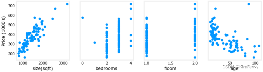
可视化，绘制每个特征和目标值的对比图，可以观察哪个特征的影响更大

fig,ax=plt.subplots(1, 4, figsize=(12, 3), sharey=True)
for i in range(len(ax)):
    ax[i].scatter(X_train[:,i],y_train)
    ax[i].set_xlabel(X_features[i])
ax[0].set_ylabel("Price (1000's)")
plt.show()

2.梯度下降

Here are the equations you developed in the last lab on gradient descent for multiple variables.:

repeat  until convergence:    {    w j : = w j − α ∂ J ( w , b ) ∂ w j    for j = 0..n-1 b    : = b − α ∂ J ( w , b ) ∂ b } \begin{align*} \text{repeat}&\text{ until convergence:} \; \lbrace \newline\; & w_j := w_j - \alpha \frac{\partial J(\mathbf{w},b)}{\partial w_j} \tag{1} \; & \text{for j = 0..n-1}\newline &b\ \ := b - \alpha \frac{\partial J(\mathbf{w},b)}{\partial b} \newline \rbrace \end{align*} repeat}​ until convergence:{wj​:=wj​−α∂wj​∂J(w,b)​b  :=b−α∂b∂J(w,b)​​for j = 0..n-1(1)​

where, n is the number of features, parameters $w_j$, $b$, are updated simultaneously and where

$$\begin{array}{rl}\frac{\partial J(\mathbf{w},b)}{\partial w_j}& =\frac{1}{m}\sum _{i=0}^{m-1}(f_{\mathbf{w},b}({\mathbf{x}}^{(i)})-y^{(i)})x_j^{(i)}\\ \frac{\partial J(\mathbf{w},b)}{\partial b}& =\frac{1}{m}\sum _{i=0}^{m-1}(f_{\mathbf{w},b}({\mathbf{x}}^{(i)})-y^{(i)})\end{array}\text{\hspace{1em}(2)(3)}$$

• m is the number of training examples in the data set

• $f_{\mathbf{w},b}({\mathbf{x}}^{(i)})$ is the model’s prediction, while $y^{(i)}$ is the target value

具体理论和代码实现在【Machine Learning】3.多元线性回归 所说过

3.学习率的选择

学习率太大会无法收敛到最优值，学习率太小收敛速度慢，因此要选择一个恰当的学习率

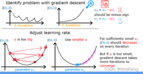
学习率太大时的图像

这个图像的代价甚至是在增长,说明学习率大得离谱

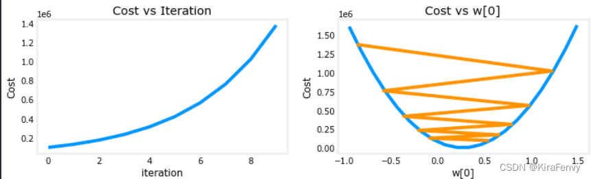
这个图像摆动幅度太大，收敛慢

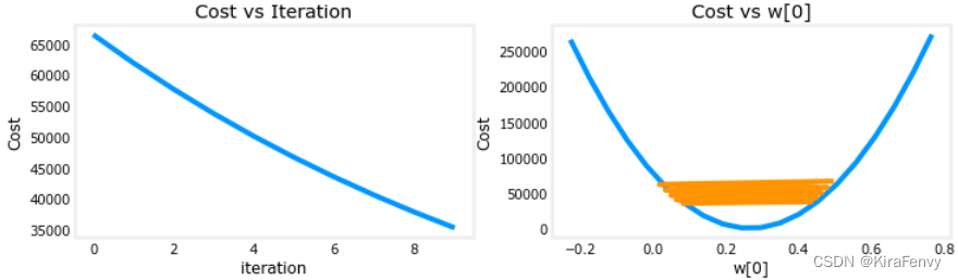
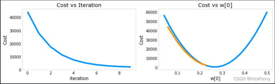
收敛速度合适的图像

4.特征缩放

三种技术：

• Feature scaling 特征缩放, essentially dividing each feature by a user selected value to result in a range between -1 and 1.
• Mean normalization 均值标准化: $$x_i:=\frac{x_i-{\mu }_i}{max-min}$$
• Z-score normalization which we will explore below. Z-score归一化

4.1 z-score normalization

After z-score normalization, all features will have a mean of 0 and a standard deviation of 1. 处理之后，特征平均值为0，标准差为1

$$x_j^{(i)}=\frac{x_j^{(i)}-{\mu }_j}{{\sigma }_j}\text{\hspace{1em}(4)}$$
where $j$ selects a feature or a column in the X matrix. ${\mu }_j$ is the mean of all the values for feature (j) and ${\sigma }_j$ is the standard deviation of feature (j).
$$\begin{array}{rl}{\mu }_j& =\frac{1}{m}\sum _{i=0}^{m-1}{x}_j^{(i)}\\ {\sigma }_j^2& =\frac{1}{m}\sum _{i=0}^{m-1}(x_j^{(i)}-{\mu }_j{)}^2\end{array}\text{\hspace{1em}(5)(6)}$$

Implementation Note: 记得把均值和方差标准差存储到变量当中

def zscore_normalize_features(X):
    """
    computes  X, zcore normalized by column
    
    Args:
      X (ndarray): Shape (m,n) input data, m examples, n features
      
    Returns:
      X_norm (ndarray): Shape (m,n)  input normalized by column
      mu (ndarray):     Shape (n,)   mean of each feature
      sigma (ndarray):  Shape (n,)   standard deviation of each feature
    """
    # find the mean of each column/feature
    mu     = np.mean(X, axis=0)                 # mu will have shape (n,)
    # find the standard deviation of each column/feature
    sigma  = np.std(X, axis=0)                  # sigma will have shape (n,)
    # element-wise, subtract mu for that column from each example, divide by std for that column
    X_norm = (X - mu) / sigma      

    return (X_norm, mu, sigma)
 
#check our work
#from sklearn.preprocessing import scale
#scale(X_orig, axis=0, with_mean=True, with_std=True, copy=True)

绘图表示处理过程：

mu     = np.mean(X_train,axis=0)   
sigma  = np.std(X_train,axis=0) 
X_mean = (X_train - mu)
X_norm = (X_train - mu)/sigma      

fig,ax=plt.subplots(1, 3, figsize=(12, 3))
ax[0].scatter(X_train[:,0], X_train[:,3])
ax[0].set_xlabel(X_features[0]); ax[0].set_ylabel(X_features[3]);
ax[0].set_title("unnormalized")
ax[0].axis('equal')

ax[1].scatter(X_mean[:,0], X_mean[:,3])
ax[1].set_xlabel(X_features[0]); ax[0].set_ylabel(X_features[3]);
ax[1].set_title(r"X - $\mu$")
ax[1].axis('equal')

ax[2].scatter(X_norm[:,0], X_norm[:,3])
ax[2].set_xlabel(X_features[0]); ax[0].set_ylabel(X_features[3]);
ax[2].set_title(r"Z-score normalized")
ax[2].axis('equal')
plt.tight_layout(rect=[0, 0.03, 1, 0.95])
fig.suptitle("distribution of features before, during, after normalization")
plt.show()

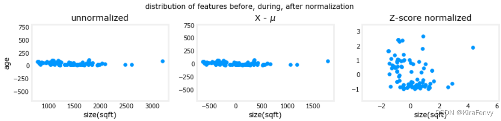
• 左：未规范化：“大小（平方英尺）”特征的值范围或方差比年龄大得多
• 中间：第一步从每个特征中减去平均值。这会留下以零为均值的特征。很难看出“年龄”特征的差异，但“大小（平方英尺）”显然约为零。
• 右：第二步除以方差。这将使两个要素以类似的比例居中于零。

计算并存储均值和标准差：

# normalize the original features
X_norm, X_mu, X_sigma = zscore_normalize_features(X_train)
print(f"X_mu = {X_mu}, \nX_sigma = {X_sigma}")
print(f"Peak to Peak range by column in Raw        X:{np.ptp(X_train,axis=0)}")   
print(f"Peak to Peak range by column in Normalized X:{np.ptp(X_norm,axis=0)}")


X_mu = [1.42e+03 2.72e+00 1.38e+00 3.84e+01], 
X_sigma = [411.62   0.65   0.49  25.78]
Peak to Peak range by column in Raw        X:[2.41e+03 4.00e+00 1.00e+00 9.50e+01]
Peak to Peak range by column in Normalized X:[5.85 6.14 2.06 3.69]

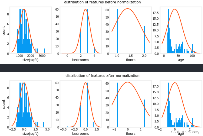
绘制归一化前和归一化后的各个特征的分布

fig,ax=plt.subplots(1, 4, figsize=(12, 3))
for i in range(len(ax)):
    norm_plot(ax[i],X_train[:,i],)
    ax[i].set_xlabel(X_features[i])
ax[0].set_ylabel("count");
fig.suptitle("distribution of features before normalization")
plt.show()
fig,ax=plt.subplots(1,4,figsize=(12,3))
for i in range(len(ax)):
    norm_plot(ax[i],X_norm[:,i],)
    ax[i].set_xlabel(X_features[i])
ax[0].set_ylabel("count"); 
fig.suptitle(f"distribution of features after normalization")

plt.show()

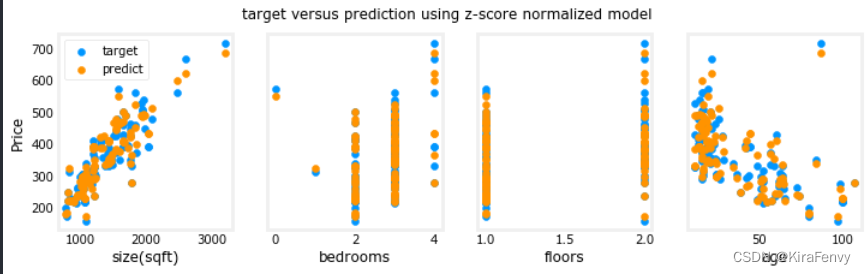
最后用归一化的数据再做一次梯度下降

w_norm, b_norm, hist = run_gradient_descent(X_norm, y_train, 1000, 1.0e-1, )

请注意，使用标准化特征进行预测，而使用原始特征值显示绘图。

#predict target using normalized features
m = X_norm.shape[0]
yp = np.zeros(m)
for i in range(m):  #使用标准化特征预测
    yp[i] = np.dot(X_norm[i], w_norm) + b_norm

    # plot predictions and targets versus original features    
fig,ax=plt.subplots(1,4,figsize=(12, 3),sharey=True)
for i in range(len(ax)):
    ax[i].scatter(X_train[:,i],y_train, label = 'target') #使用原始特征值绘图
    ax[i].set_xlabel(X_features[i])
    ax[i].scatter(X_train[:,i],yp,color=dlorange, label = 'predict')
ax[0].set_ylabel("Price"); ax[0].legend();
fig.suptitle("target versus prediction using z-score normalized model")
plt.show()

记得要用多个图来显示每个特征与预测值、目标值间关系

4.2.预测

预测的时候也要将输入数据进行归一化

# First, normalize out example.
x_house = np.array([1200, 3, 1, 40])
x_house_norm = (x_house - X_mu) / X_sigma
print(x_house_norm)
x_house_predict = np.dot(x_house_norm, w_norm) + b_norm
print(f" predicted price of a house with 1200 sqft, 3 bedrooms, 1 floor, 40 years old = ${x_house_predict*1000:0.0f}")


[-0.53  0.43 -0.79  0.06]
 predicted price of a house with 1200 sqft, 3 bedrooms, 1 floor, 40 years old = $318709

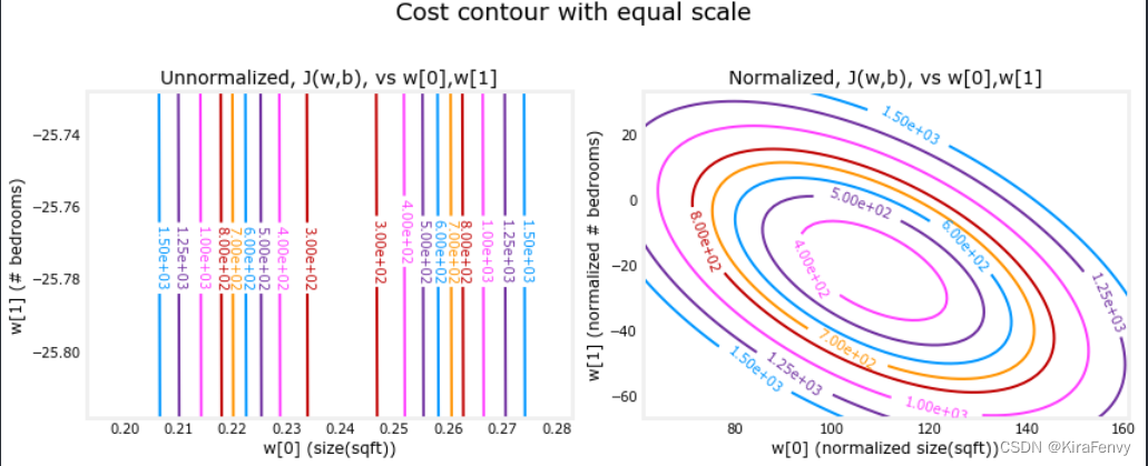
4.3 代价等高线 cost contours

当特征比例不匹配时，等高线图中成本与参数的关系图是不对称的。

在下图中，参数的比例是匹配的。左边的图是w[0]的成本等值线图，平方英尺与w[1]的对比，是特征正常化之前的卧室数量。图是如此不对称，完成轮廓的曲线是不可见的。相比之下，当特征归一化时，成本轮廓更加对称。结果是，梯度下降期间的参数更新可以使每个参数的进度相等。