


在上一篇文章中已经介绍了Pytorch中Dataset类以及Transform类中一些方法的使用,接下来介绍利用Pytorch来实现卷积等操作的实现。
一、nn.Module类
一个nn.Module是神经网络的基本骨架,可以视为一个块。如果神经网络要重写初始方法,则必须要调用父类的初始化函数。
所有的module包含两个主要函数:
init函数:在里边定义一些需要的类或参数。包括网络层。
forward函数:做最终的计算和输出,其形参就是模型(块)的输入。
现在来简单写一个类:
class Test1(nn.Module):
def __init__(self) -> None:
super().__init__()
def forward(self,input):
output = input+1
return output
这个类的作用是传入一个数,输出这个数加一后的结果,调用类:
test1 = Test1()

x = torch.tensor(1.0)
注意:在调用forward方法时不用引用函数,因为集成的nn.Module中的forward方法是__call__()方法的实现,可调用对象会调用__call__()方法。
output = test1(x)

print(output)
输出结果如下:

二、卷积
1、conv2d
卷积分为不同的层,如con1、con2等,以二层卷积为例,具体的参数可查看官方文档,卷积操作主要就是用卷积核(weight)与原始数据进行计算,再加上其他的操作,最后得到一个新的输出。。
其中一些重要参数的含义如下:
output就是卷积神经网络模型计算后的输出。
input是输入的数据,在此为一个二维数组,代表一张图片。
kernel表示卷积核,同input形状,也是一个二维数组,并且两者的形状都要有四个指标,否则要进行reshape。
stride表示步长。
padding表示周围填充几层,填充的默认值是0。
首先导入包:
import torch

import torch.nn.functional as F
设置输入数据:
input = torch.tensor([[1, 2, 0, 3, 1],

                      [0, 1, 2, 3, 1],

                      [1, 2, 1, 0, 0],

                      [5, 2, 3, 1, 1],

                      [2, 1, 0, 1, 1]])
设置卷积核:
kernel = torch.tensor([[1, 2, 1],

                       [0, 1, 0],

                       [2, 1, 0]])
因为设置的数据并不完整,所以进行reshape
input = torch.reshape(input, (1, 1, 5, 5))

kernel = torch.reshape(kernel, (1, 1, 3, 3))
进行步长为1的卷积:
output1 = F.conv2d(input, kernel, stride=1)

print(output1)
输出结果如下:

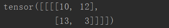
进行步长为2的卷积:
output2 = F.conv2d(input, kernel, stride=2)

print(output2)
输出结果如下:
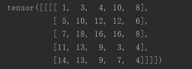
进行步长为1,填充层为1的卷积:
output3 = F.conv2d(input, kernel, stride=1, padding=1)

print(output3)
输出结果如下:
2、Conv2d
其实就是对nn.function的进一步封装,如nn.Conv2(),最常用的是这五个参数:in_channels、 out_channels、kernel_size、stride、padding
首先导入需要的包:
import torch

import torchvision

from torch import nn

from torch.nn import Conv2d

from torch.utils.data import DataLoader

from torch.utils.tensorboard import SummaryWriter
使用dataset下载需要用到的训练样本,并且使用dataloader进行封装:
dataset = torchvision.datasets.CIFAR10('dataset', train=False, transform=torchvision.transforms.ToTensor(),download=True)

dataloader = DataLoader(dataset, batch_size=64)
构造类:
class Test1(nn.Module):

    def __init__(self):

        super(Test1, self).__init__()

        # 因为是彩色图像,所以in_channels=3,输出通道数=6

        self.conv1 = Conv2d(in_channels=3, out_channels=6, kernel_size=3, stride=1, padding=0)


    def forward(self, x):

        x = self.conv1(x)

        return x
此时,设置的卷积核大小为3x3,输出通道数为6。
调用类,将训练样本传入类,并在浏览器中显示:
test1 = Test1()

step = 0

writer = SummaryWriter('logs_conv2d')

for data in dataloader:

    imgs, targets = data

    output = test1(imgs)
# 传入卷积前的图像,torch.Size([64, 3, 32, 32])

    writer.add_images('iuput', imgs, step)

    # 传入卷积后的图像,torch.Size([64, 6, 30, 30])

    # 卷积后的图像channel数为6,无法显示图像

    output = torch.reshape(output, (-1, 3, 30, 30))

    writer.add_images('output', output, step)

    step = step + 1

writer.close()
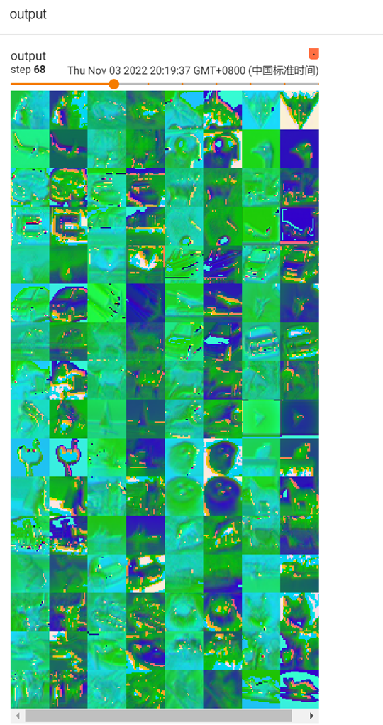
输出结果如下:
Input为原始图像:

Output为卷积后的图像:
三、最大池化
最大池化层(常用的是maxpool2d)的作用:
一是对卷积层所提取的信息做更一步降维,减少计算量。
二是加强图像特征的不变性,使之增加图像的偏移、旋转等方面的鲁棒性。
三是类似于观看视频时不同的清晰度,实际效果就像给图片打马赛克。
1、对二维数组进行最大池化
首先导入包:
import torch

from torch import nn

from torch.nn import MaxPool2d
定义一个二位tensor类数组:
input = torch.tensor([[1, 2, 0, 3, 1],

                      [0, 1, 2, 3, 1],

                      [1, 2, 1, 0, 0],

                      [5, 2, 3, 1, 1],

                      [2, 1, 0, 1, 1]], dtype=torch.float32)
进行reshape:
input = torch.reshape(input, (-1, 1, 5, 5))
定义进行最大池化的类:
class Test1(nn.Module):

    def __init__(self):

        super(Test1, self).__init__()

        self.maxpool1 = MaxPool2d(kernel_size=3, ceil_mode=True)


    def forward(self, input):

        output = self.maxpool1(input)

        return output
以上,滤波器为3x3,ceil_mode为True时,不舍弃多余的像素,在不满足3x3的原数组边加零。
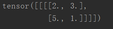
调用类:
test1 = Test1()

output = test1(input)

print(output)
输出结果如下:
2、对图像进行最大池化
首先导入包:
import torchvision

from torch import nn

from torch.nn import MaxPool2d

from torch.utils.data import DataLoader

from torch.utils.tensorboard import SummaryWriter
使用dataset下载需要用到的训练样本,并且使用dataloader进行封装:
dataset = torchvision.datasets.CIFAR10('dataset', train=False, transform=torchvision.transforms.ToTensor(),download=True)

dataloader = DataLoader(dataset, batch_size=64)
构造类:
class Test1(nn.Module):

    def __init__(self):

        super(Test1, self).__init__()

        self.maxpool1 = MaxPool2d(kernel_size=3, ceil_mode=True)

    def forward(self, input):

        output = self.maxpool1(input)

        return output
调用类:
test1 = Test1()

step = 0

writer = SummaryWriter('logs_maxpool')

for data in dataloader:

    imgs, targets = data

    output = test1(imgs)

    writer.add_images('iuput', imgs, step)

    writer.add_images('output', output, step)

    step = step + 1


writer.close()
输出结果如下:
原始图像如下:

经最大池化后的图像如下:

四、非线性激活
非线性变换的主要目的就是给网中加入一些非线性特征,非线性越多才能训练出符合各种特征的模型。常见的非线性激活:
ReLU:主要是对小于0的进行截断(将小于0的变为0),图像变换效果不明显。主要参数是inplace:
inplace为真时,将处理后的结果赋值给原来的参数;为假时,原值不会改变。
Sigmoid: 归一化处理。效果没有ReLU好,但对于多远分类问题,必须采用sigmoid。
以ReLU方法为例:
首先导入包
import torch

from torch import nn

from torch.nn import ReLU
设置传入参数:
input = torch.tensor([[1, -0.5],

                      [-1, 3]])

input = torch.reshape(input, (-1, 1, 2, 2))
构造类:
class Test1(nn.Module):

    def __init__(self):

        super(Test1, self).__init__()

        self.relu1 = ReLU()

    def forward(self, input):

        output = self.relu1(input)

        return output
调用类:
test1 = Test1()

output = test1(input)

print(output)
输出结果如下:

五、线性层
线性层又叫全连接层,其中每个神经元与上一层所有神经元相连。
线性函数为:torch.nn.Linear(in_features, out_features, bias=True, device=None, dtype=None),其中重要的3个参数in_features、out_features、bias说明如下:
in_features:每个输入(x)样本的特征的大小
out_features:每个输出(y)样本的特征的大小
bias:如果设置为False,则图层不会学习附加偏差。默认值是True,表示增加学习偏置。
在上图中,in_features=d,out_features=L。
作用可以是缩小一维的数据长度。
- Sequential的使用(torch.nn.Sequential)
可以将所需要的操作全部写在一个函数中。主要是方便代码的编写,使代码更加简洁。
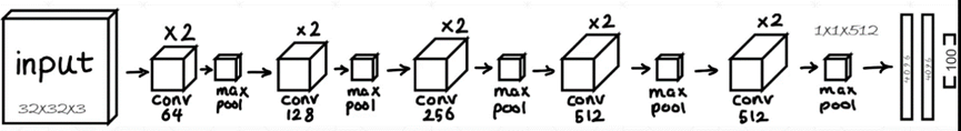
例如实现如下图所示模型:
首先导入包:
import torch

from torch import nn

from torch.nn import Conv2d, MaxPool2d, Flatten, Linear, Sequential

from torch.utils.tensorboard import SummaryWriter
构造类:
class Test(nn.Module):

    def __init__(self):

        super(Test, self).__init__()

        self.model1 = Sequential(

            Conv2d(in_channels=3, out_channels=32, kernel_size=5, stride=1, padding=2),

            MaxPool2d(2),

            Conv2d(in_channels=32, out_channels=32, kernel_size=5, padding=2, stride=1),

            MaxPool2d(2),

            Conv2d(in_channels=32, out_channels=64, kernel_size=5, padding=2, stride=1),

            MaxPool2d(2),

            Flatten(),

            Linear(in_features=1024, out_features=64),

            Linear(in_features=64, out_features=10)

        )


    def forward(self, x):

        x = self.model1(x)

        return x
调用类:
test1 = Test()

print(test1)

input = torch.ones((64, 3, 32, 32))

output = test1(input)

print(output.shape)


writer = SummaryWriter('logs_seq1')

writer.add_graph(test1, input)

writer.close()
输出结果如下:
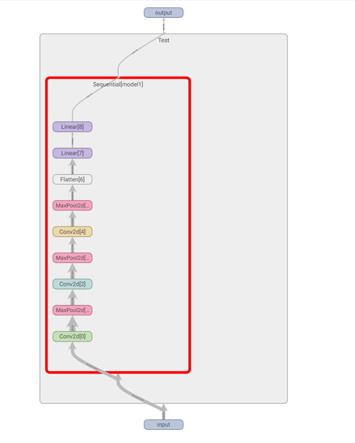
可以看到这个神经网络模型的脉络。


 1034
1034


 被折叠的 条评论
为什么被折叠?
被折叠的 条评论
为什么被折叠?
 到【灌水乐园】发言


