BP神经网络学习笔记8.29

一 认识BP神经网络

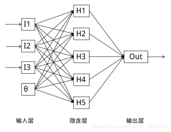
经典的BP神经网络通常由三层组成: 输入层， 隐含层与输出层.通常输入层神经元的个数与特征数相关，输出层的个数与类别数相同， 隐含层的层数与神经元数均可以自定义.

 

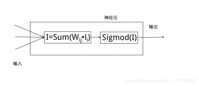
每个神经元代表对数据的一次处理:

 

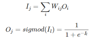
每个隐含层和输出层神经元输出与输入的函数关系为:

二 BP神经网络结构与原理

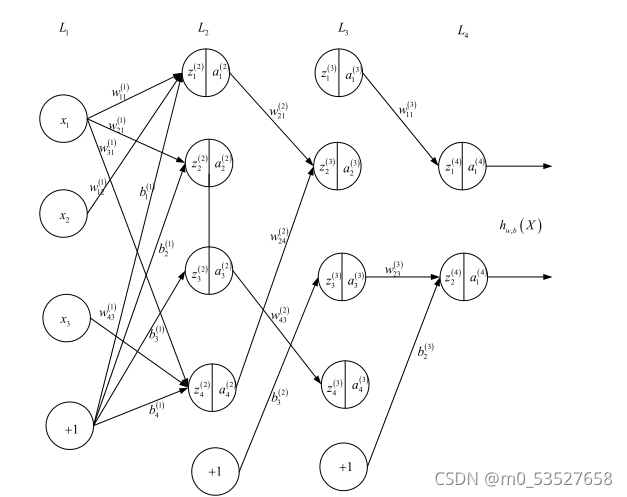
 由于 BP 神经网络参数超级多，如果不先定义好变量，后面非常难理解，故针对上述图
形，定义如下：

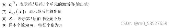
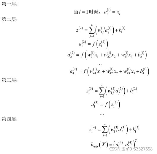
 通过上面的定义可知：

三 BP神经网络的第一种实现

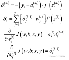
采用误差平方和作为损失函数，基于反向传播算法推导，可得最终的 4 个方程式，如下：

 

 

 3.1 前向计算

 

        for b, w in zip(self.biases, self.weights):
            z = np.dot(w, activation) + b
            zs.append(z)
            activation = sigmoid(z)
            activations.append(activation)

3.2 反向传播

# backward pass 计算最后一层的误差
        delta = self.cost_derivative(activations[-1], y) * \
                sigmoid_prime(zs[-1])
        nabla_b[-1] = delta
        nabla_w[-1] = np.dot(delta, activations[-2].transpose())
        # 计算从倒数第二层至第二层的误差
        for l in range(2, self.num_layers):
            z = zs[-l]
            sp = sigmoid_prime(z)
            delta = np.dot(self.weights[-l + 1].transpose(), delta) * sp
            nabla_b[-l] = delta
            nabla_w[-l] = np.dot(delta, activations[-l - 1].transpose())

四 BP神经网络的第二种实现

4.1 交叉熵代价函数
“严重错误”导致学习缓慢，如果在初始化权重和偏置时，故意产生一个背离预期较大的
输出，那么训练网络的过程中需要用很多次迭代，才能抵消掉这种背离，恢复正常的学习。
(1) 引入交叉熵代价函数目的是解决一些实例在刚开始训练时学习得非常慢的问题，其
主要针对激活函数为 Sigmod 函数
(2) 如果采用一种不会出现饱和状态的激活函数，那么可以继续使用误差平方和作为损
失函数
(3) 如果在输出神经元是 S 型神经元时 ， 交叉熵 一 般都是更好的选择
(4) 输出神经元是线性的那么二次代价函数不再会导致学习速度下降的问题。在此情形
下，二次代价函数就是一种合适的选择
(5) 交叉熵无法改善隐藏层中神经元发生的学习缓慢
(6) 交叉熵损失函数只对网络输出“ 明显背离预期” 时发生的学习缓慢有改善效果
(7) 应用交叉熵损失并不能改善或避免神经元饱和 ，而是当输出层神经元发生饱和时，
能够避免其学习缓慢的问题。
4.2 种规范化技术
(1) 早停止。跟踪验证数据集上的准确率随训练变化情况。如果我们看到验证数据上的
准确率不再提升，那么我们就停止训练
(2) 正则化
(3) 弃权( Dropout )
(4) 扩增样本集
4.3 更好的权重初始化方法
不好的权重初始化方法会导致出现饱和问题，好的权重初始化方法不仅仅能够带来训练
速度的加快，有时候在最终性能上也有很大的提升

代码实现：

主要代码：

class QuadraticCost(object): # 误差平方和代价函数
 
    @staticmethod
    def fn(a, y):
        """Return the cost associated with an output ``a`` and desired output
        ``y``.
        """
        return 0.5*np.linalg.norm(a-y)**2
 
    @staticmethod
    def delta(z, a, y):
        """Return the error delta from the output layer."""
        return (a-y) * sigmoid_prime(z)
 
 
class CrossEntropyCost(object): # 交叉熵代价函数
 
    @staticmethod
    def fn(a, y):
        """Return the cost associated with an output ``a`` and desired output
        ``y``.  Note that np.nan_to_num is used to ensure numerical
        stability.  In particular, if both ``a`` and ``y`` have a 1.0
        in the same slot, then the expression (1-y)*np.log(1-a)
        returns nan.  The np.nan_to_num ensures that that is converted
        to the correct value (0.0).
        """
        return np.sum(np.nan_to_num(-y*np.log(a)-(1-y)*np.log(1-a))) # 使用0代替nan 一个较大值代替inf

#### Libraries
# Standard library
import json
import random
import sys
# Third-party libraries
import numpy as np
#### Define the quadratic and cross-entropy cost functions
import mnist_loader
 
 
class QuadraticCost(object): # 误差平方和代价函数
 
    @staticmethod
    def fn(a, y):
        return 0.5*np.linalg.norm(a-y)**2
 
    @staticmethod
    def delta(z, a, y):
        """Return the error delta from the output layer."""
        return (a-y) * sigmoid_prime(z)
 
 
class CrossEntropyCost(object): # 交叉熵代价函数
 
    @staticmethod
    def fn(a, y):
        return np.sum(np.nan_to_num(-y*np.log(a)-(1-y)*np.log(1-a))) # 使用0代替nan 一个较大值代替inf
 
    @staticmethod
    def delta(z, a, y):
        return (a-y)
 
 
#### Main Network class
class Network(object):
 
    def __init__(self, sizes, cost=CrossEntropyCost):  #采用交叉熵代价函数
 
        self.num_layers = len(sizes)
        self.sizes = sizes
        self.default_weight_initializer()
        self.cost=cost
 
    def default_weight_initializer(self): # 推荐的权重初始化方式
        self.biases = [np.random.randn(y, 1) for y in self.sizes[1:]] # 偏差初始化方式不变
        self.weights = [np.random.randn(y, x)/np.sqrt(x)  # 将方差减少，避免饱和
                        for x, y in zip(self.sizes[:-1], self.sizes[1:])]
 
    def large_weight_initializer(self): # 不推荐的初始化方式
        self.biases = [np.random.randn(y, 1) for y in self.sizes[1:]]
        self.weights = [np.random.randn(y, x)
                        for x, y in zip(self.sizes[:-1], self.sizes[1:])]
 
    def feedforward(self, a):
        """Return the output of the network if ``a`` is input."""
        for b, w in zip(self.biases, self.weights):
            a = sigmoid(np.dot(w, a)+b)
        return a
 
    def SGD(self, training_data, epochs, mini_batch_size, eta,
            lmbda = 0.0,
            evaluation_data=None,
            monitor_evaluation_cost=False,
            monitor_evaluation_accuracy=False,
            monitor_training_cost=False,
            monitor_training_accuracy=False,
            early_stopping_n = 0):
        # early stopping functionality:
        best_accuracy=1
 
        training_data = list(training_data)
        n = len(training_data)
 
        if evaluation_data:
            evaluation_data = list(evaluation_data)
            n_data = len(evaluation_data)
 
        # early stopping functionality:
        best_accuracy=0
        no_accuracy_change=0
 
        evaluation_cost, evaluation_accuracy = [], []
        training_cost, training_accuracy = [], []
        for j in range(epochs):
            random.shuffle(training_data)
            mini_batches = [
                training_data[k:k+mini_batch_size]
                for k in range(0, n, mini_batch_size)]
            for mini_batch in mini_batches:
                self.update_mini_batch(
                    mini_batch, eta, lmbda, len(training_data))
 
            print("Epoch %s training complete" % j)
 
            if monitor_training_cost:
                cost = self.total_cost(training_data, lmbda)
                training_cost.append(cost)
                print("Cost on training data: {}".format(cost))
            if monitor_training_accuracy:
                accuracy = self.accuracy(training_data, convert=True)
                training_accuracy.append(accuracy)
                print("Accuracy on training data: {} / {}".format(accuracy, n))
            if monitor_evaluation_cost:
                cost = self.total_cost(evaluation_data, lmbda, convert=True)
                evaluation_cost.append(cost)
                print("Cost on evaluation data: {}".format(cost))
            if monitor_evaluation_accuracy:
                accuracy = self.accuracy(evaluation_data)
                evaluation_accuracy.append(accuracy)
                print("Accuracy on evaluation data: {} / {}".format(self.accuracy(evaluation_data), n_data))
 
            # Early stopping:
            if early_stopping_n > 0: # 如果采用了早停止策略，则当准确率超过设定的次数依然没有改变，则停止训练
                if accuracy > best_accuracy:
                    best_accuracy = accuracy
                    no_accuracy_change = 0
                    print("Early-stopping: Best so far {}".format(best_accuracy))
                else:
                    no_accuracy_change += 1
 
                if (no_accuracy_change == early_stopping_n):
                    print("Early-stopping: No accuracy change in last epochs: {}".format(early_stopping_n))
                    return evaluation_cost, evaluation_accuracy, training_cost, training_accuracy
 
        return evaluation_cost, evaluation_accuracy, \
            training_cost, training_accuracy
 
    def update_mini_batch(self, mini_batch, eta, lmbda, n):
        nabla_b = [np.zeros(b.shape) for b in self.biases]
        nabla_w = [np.zeros(w.shape) for w in self.weights]
        for x, y in mini_batch:
            delta_nabla_b, delta_nabla_w = self.backprop(x, y)
            nabla_b = [nb+dnb for nb, dnb in zip(nabla_b, delta_nabla_b)]
            nabla_w = [nw+dnw for nw, dnw in zip(nabla_w, delta_nabla_w)]
        self.weights = [(1-eta*(lmbda/n))*w-(eta/len(mini_batch))*nw # 带L2范数的权重更新
                        for w, nw in zip(self.weights, nabla_w)]
        self.biases = [b-(eta/len(mini_batch))*nb
                       for b, nb in zip(self.biases, nabla_b)]
 
    def backprop(self, x, y):
        nabla_b = [np.zeros(b.shape) for b in self.biases]
        nabla_w = [np.zeros(w.shape) for w in self.weights]
        # feedforward
        activation = x
        activations = [x] # list to store all the activations, layer by layer
        zs = [] # list to store all the z vectors, layer by layer
        for b, w in zip(self.biases, self.weights):
            z = np.dot(w, activation)+b
            zs.append(z)
            activation = sigmoid(z)
            activations.append(activation)
        # backward pass
        delta = (self.cost).delta(zs[-1], activations[-1], y) # 这里和以前不一样，其他地方一样
        nabla_b[-1] = delta
        nabla_w[-1] = np.dot(delta, activations[-2].transpose())
        # Note that the variable l in the loop below is used a little
        # differently to the notation in Chapter 2 of the book.  Here,
        # l = 1 means the last layer of neurons, l = 2 is the
        # second-last layer, and so on.  It's a renumbering of the
        # scheme in the book, used here to take advantage of the fact
        # that Python can use negative indices in lists.
        for l in range(2, self.num_layers):
            z = zs[-l]
            sp = sigmoid_prime(z)
            delta = np.dot(self.weights[-l+1].transpose(), delta) * sp
            nabla_b[-l] = delta
            nabla_w[-l] = np.dot(delta, activations[-l-1].transpose())
        return (nabla_b, nabla_w)
 
    def accuracy(self, data, convert=False):
        if convert: # 训练集使用-由于训练集的输出是独热码，而其他数据不是
            results = [(np.argmax(self.feedforward(x)), np.argmax(y))
                       for (x, y) in data]
        else: # 验证集合测试集使用
            results = [(np.argmax(self.feedforward(x)), y)
                        for (x, y) in data]
 
        result_accuracy = sum(int(x == y) for (x, y) in results)
        return result_accuracy
 
    def total_cost(self, data, lmbda, convert=False):
        cost = 0.0
        for x, y in data:
            a = self.feedforward(x)
            if convert: y = vectorized_result(y) # 测试集和验证集需要向量化
            cost += self.cost.fn(a, y)/len(data) # 带L2范数的代价函数
            cost += 0.5*(lmbda/len(data))*sum(np.linalg.norm(w)**2 for w in self.weights) # '**' - to the power of.
        return cost
 
    def save(self, filename):
        data = {"sizes": self.sizes,
                "weights": [w.tolist() for w in self.weights],
                "biases": [b.tolist() for b in self.biases],
                "cost": str(self.cost.__name__)}
        f = open(filename, "w")
        json.dump(data, f)
        f.close()
 
#### Loading a Network
def load(filename):
    f = open(filename, "r")
    data = json.load(f)
    f.close()
    cost = getattr(sys.modules[__name__], data["cost"])
    net = Network(data["sizes"], cost=cost)
    net.weights = [np.array(w) for w in data["weights"]]
    net.biases = [np.array(b) for b in data["biases"]]
    return net
 
#### Miscellaneous functions
def vectorized_result(j):
    e = np.zeros((10, 1))
    e[j] = 1.0
    return e
 
def sigmoid(z):
    """The sigmoid function."""
    return 1.0/(1.0+np.exp(-z))
 
def sigmoid_prime(z):
    """Derivative of the sigmoid function."""
    return sigmoid(z)*(1-sigmoid(z))
 
if __name__ == '__main__':
 
    training_data, validation_data, test_data = mnist_loader.load_data_wrapper()
    training_data = list(training_data)
 
    net = Network([784, 30, 10], cost=CrossEntropyCost)
    # net.large_weight_initializer()
    net.SGD(training_data, 30, 10, 0.1, lmbda=5.0, evaluation_data=validation_data,
            monitor_evaluation_accuracy=True)