


本数据集的下载地址,读者可以自行下载。
公众号(可以与我取得联系):蓝皮怪的数据坊
知乎:知乎ID—蓝皮怪
CSDN:CSDN—蓝皮怪
1.项目背景
随着社会的发展和大众对数据的重视,警察和警犬的伤亡数据成为了执法部门、分析师以及研究人员关注的重要信息,基于对1791年至2022年间美国警察及1877年至2022年间警犬的死亡数据进行全面分析,可以更好地理解警察和警犬在执法过程中的表现及其所面临的风险,继而为相关部门制定保护措施和政策提供数据支持。
2.数据说明
警察数据:
| 字段 | 说明 |
|---|---|
| Rank | 警察在其任职期间被授予或达到的职级 |
| Name | 姓名 |
| Age | 年龄 |
| End_Of_Watch | 被宣布死亡的日期 |
| Day_Of_Week | 当天星期几 |
| Cause | 死亡原因 |
| Department | 工作的部门名称 |
| State | 部门所在州 |
| Tour | 任职期限 |
| Badge | 徽章编号 |
| Weapon | 导致警官死亡的武器 |
| Offender | 犯罪者/凶手;此字段说明了事件后犯罪者的下场,例如被捕、被击毙等 |
| Summary | 警察的简介以及事件摘要,包括发生了什么、警察是如何死亡的等等 |
警犬数据:
| 字段 | 说明 |
|---|---|
| Rank | 警犬在其任职期间被授予或达到的等级 |
| Name | 警犬名字 |
| Breed | 警犬品种 |
| Gender | 警犬性别 |
| Age | 警犬年龄 |
| End_Of_Watch | 警犬被宣布死亡的日期 |
| Day_Of_Week | 当天星期几 |
| Cause | 警犬死亡原因 |
| Department | 警犬所属部门名称 |
| State | 部门所在州 |
| Tour | 警犬任职期限 |
| Weapon | 导致警犬死亡的武器 |
| Offender | 犯罪者/凶手;此字段说明了事件后犯罪者的下场,例如被捕、被击毙等 |
| Summary | 警犬的简介以及事件摘要,包括发生了什么、它是如何死亡的等等 |
3.Python库导入及数据读取
import pandas as pd
import numpy as np
import seaborn as sns
import matplotlib.pyplot as plt
import matplotlib.ticker as mticker
from scipy.stats import chi2_contingency
import json
# 设置显示选项
pd.set_option('display.max_columns', None)  # 显示所有列
pd.set_option('display.max_rows', None)     # 显示所有行
pd.set_option('display.max_colwidth', None) # 全局解除显示限制
police_data = pd.read_csv("/home/mw/input/12027546/police_deaths_USA.csv")
dog_data = pd.read_csv("/home/mw/input/12027546/k9_deaths_USA.csv")
4.数据预览及数据预处理
print('查看警察数据信息:')
police_data.info()
查看警察数据信息:
<class 'pandas.core.frame.DataFrame'>
RangeIndex: 25638 entries, 0 to 25637
Data columns (total 13 columns):
 #   Column        Non-Null Count  Dtype
---  ------        --------------  -----
 0   Rank          25638 non-null  object
 1   Name          25638 non-null  object
 2   Age           22959 non-null  float64
 3   End_Of_Watch  25638 non-null  object
 4   Day_Of_Week   25638 non-null  object
 5   Cause         25637 non-null  object
 6   Department    25638 non-null  object
 7   State         25638 non-null  object
 8   Tour          17432 non-null  object
 9   Badge         7486 non-null   object
 10  Weapon        16269 non-null  object
 11  Offender      13808 non-null  object
 12  Summary       25638 non-null  object
dtypes: float64(1), object(12)
memory usage: 2.5+ MB
print('查看警犬数据信息:')
dog_data.info()
查看警犬数据信息:
<class 'pandas.core.frame.DataFrame'>
RangeIndex: 506 entries, 0 to 505
Data columns (total 14 columns):
 #   Column        Non-Null Count  Dtype
---  ------        --------------  -----
 0   Rank          506 non-null    object
 1   Name          506 non-null    object
 2   Breed         505 non-null    object
 3   Gender        447 non-null    object
 4   Age           341 non-null    float64
 5   End_Of_Watch  506 non-null    object
 6   Day_Of_Week   506 non-null    object
 7   Cause         506 non-null    object
 8   Department    506 non-null    object
 9   State         506 non-null    object
 10  Tour          230 non-null    object
 11  Weapon        230 non-null    object
 12  Offender      172 non-null    object
 13  Summary       506 non-null    object
dtypes: float64(1), object(13)
memory usage: 55.5+ KB
这里说一下,我处理缺失值比较莽撞的做法,我一开始考虑用正则或者NLP从Summary里提取信息去填充到Weapon和Offender,虽然有一定成效,但是耗时2天搞出来后才发现,我根本不需要知道凶手的下场、凶器情况,因为Cause已经能够说明该警员死亡的原因了,所以后续我处理缺失值,打算直接删除Name、Tour、Weapon、Offender、Summary,然后针对数据中缺少的年龄数据,暂时不先处理,因为做描述性统计的时候不会影响。
police_data[police_data['Cause'].isnull()]
| Rank | Name | Age | End_Of_Watch | Day_Of_Week | Cause | Department | State | Tour | Badge | Weapon | Offender | Summary | |
|---|---|---|---|---|---|---|---|---|---|---|---|---|---|
| 2297 | Chief of Police | Hansford P. Gipson | 56.0 | 1901-10-14 | Monday | NaN | Tuscumbia Police Department, Alabama | Alabama | NaN | NaN | NaN | NaN | Chief Gipson suffered a stroke and died as he escorted a prisoner to jail. Another officer saw his chief fall. He and the prisoner removed the chief to the jail where he was pronounced dead.Chief Gipson was survived by his wife. He was a Civil War veteran having served as a private with the 11th Alabama Calvary, Company C. |
先查看Cause缺失的那一行,看看怎么处理,可以看到是由于中风死亡的。
dog_data[dog_data['Breed'].isnull()]
| Rank | Name | Breed | Gender | Age | End_Of_Watch | Day_Of_Week | Cause | Department | State | Tour | Weapon | Offender | Summary | |
|---|---|---|---|---|---|---|---|---|---|---|---|---|---|---|
| 85 | K9 | Major | NaN | NaN | NaN | 1990-11-29 | Thursday | Struck by vehicle | Florida Highway Patrol, Florida | Florida | 1 year | NaN | NaN | K9 Major was struck and killed by a car while conducting a vehicle search on the side of a road. |
这条名为Major的警犬是在搜寻时,被汽车撞死的,通过这条消息,判断不了该警犬的品种,因此在后续分析时,可以填充为“Unknown”。
print(f'查看警察数据中的重复值:{police_data.duplicated().sum()}')
print(f'查看警犬数据中的重复值:{dog_data.duplicated().sum()}')
查看警察数据中的重复值:0
查看警犬数据中的重复值:0
characteristic = police_data.select_dtypes(include=['object']).columns.tolist()
for i in characteristic:
    print(f'警察数据中{i}:')
    print(f'共有:{len(police_data[i].unique())}条唯一值')
    print('-'*50)
警察数据中Rank:
共有:620条唯一值
--------------------------------------------------
警察数据中Name:
共有:25508条唯一值
--------------------------------------------------
警察数据中End_Of_Watch:
共有:18856条唯一值
--------------------------------------------------
警察数据中Day_Of_Week:
共有:7条唯一值
--------------------------------------------------
警察数据中Cause:
共有:37条唯一值
--------------------------------------------------
警察数据中Department:
共有:7231条唯一值
--------------------------------------------------
警察数据中State:
共有:58条唯一值
--------------------------------------------------
警察数据中Tour:
共有:371条唯一值
--------------------------------------------------
警察数据中Badge:
共有:4081条唯一值
--------------------------------------------------
警察数据中Weapon:
共有:137条唯一值
--------------------------------------------------
警察数据中Offender:
共有:1764条唯一值
--------------------------------------------------
警察数据中Summary:
共有:25605条唯一值
--------------------------------------------------
print("警察数据中Department的唯一值情况:")
print(police_data['Department'].unique())
警察数据中Department的唯一值情况:
["Albany County Constable's Office, New York"
 "Columbia County Sheriff's Office, New York"
 "Westchester County Sheriff's Department, New York" ...
 "San Jacinto County Constable's Office - Precinct 1, Texas"
 'United States Department of Defense - Marine Corps Mountain Warfare Training Center Bridgeport Police, U.S. Government'
 'Vidor Police Department, Texas']
可以发现Department其实对后续的分析意义也不大,因为数据中已经有State来表示地区了,而Department有7231条唯一值,State已经够用了。
police_data = police_data.drop(columns=["Department"])
print("警察数据中Cause的唯一值情况:")
print(police_data['Cause'].unique())
警察数据中Cause的唯一值情况:
['Stabbed' 'Gunfire' 'Duty related illness' 'Assault' 'Fall' 'Drowned'
 'Structure collapse' 'Fire' 'Gunfire (Inadvertent)' 'Explosion'
 'Vehicular assault' 'Animal related' 'Heart attack'
 'Weather/Natural disaster' 'Accidental' 'Hypothermia' 'Heatstroke'
 'Train accident' 'Struck by streetcar' 'Struck by train' 'Bomb'
 'Poisoned' 'Electrocuted' 'Boating accident' 'Bicycle accident'
 'Automobile crash' 'Struck by vehicle' nan 'Exposure to toxins'
 'Motorcycle crash' 'Vehicle pursuit' 'Unidentified' 'Training accident'
 'Aircraft accident' 'Terrorist attack' '9/11 related illness' 'COVID19']
可以将Cause缺失的那个数据归为Duty related illness(因职责相关的疾病),可能由工作压力或长期与工作相关的健康状况导致的。
police_data['Cause'] = police_data['Cause'].fillna("Duty related illness")
characteristic = dog_data.select_dtypes(include=['object']).columns.tolist()
for i in characteristic:
    print(f'警犬数据中{i}:')
    print(f'共有:{len(dog_data[i].unique())}条唯一值')
    print('-'*50)
警犬数据中Rank:
共有:1条唯一值
--------------------------------------------------
警犬数据中Name:
共有:396条唯一值
--------------------------------------------------
警犬数据中Breed:
共有:21条唯一值
--------------------------------------------------
警犬数据中Gender:
共有:3条唯一值
--------------------------------------------------
警犬数据中End_Of_Watch:
共有:483条唯一值
--------------------------------------------------
警犬数据中Day_Of_Week:
共有:7条唯一值
--------------------------------------------------
警犬数据中Cause:
共有:24条唯一值
--------------------------------------------------
警犬数据中Department:
共有:391条唯一值
--------------------------------------------------
警犬数据中State:
共有:45条唯一值
--------------------------------------------------
警犬数据中Tour:
共有:41条唯一值
--------------------------------------------------
警犬数据中Weapon:
共有:31条唯一值
--------------------------------------------------
警犬数据中Offender:
共有:41条唯一值
--------------------------------------------------
警犬数据中Summary:
共有:506条唯一值
--------------------------------------------------
同样删除Department,同时Rank只有一条唯一值,对后续分析也起不到作用,也删除,Breed有一条缺失值,根据之前的分析,用“Unknown”填充。
print('警犬数据性别唯一值:')
print(dog_data['Gender'].unique())
警犬数据性别唯一值:
['Male' nan 'Female']
同样可以用"Unknown"来填充缺失值。
dog_data['Gender'] = dog_data['Gender'].fillna("Unknown")
dog_data['Breed'] = dog_data['Breed'].fillna("Unknown Breed")
dog_data = dog_data.drop(columns=["Department","Rank"])
plt.figure(figsize=(10, 5))
plt.subplot(1, 2, 1)
# 去除 Age 列中的 NaN 值
police_age_data = police_data['Age'].dropna()
plt.boxplot(police_age_data)  # 绘制箱线图
plt.title("警察年龄的箱线图")
plt.ylabel("年龄")

plt.subplot(1, 2, 2)
dog_age_data = dog_data['Age'].dropna()
plt.boxplot(dog_age_data)  # 绘制箱线图
plt.title("警犬年龄的箱线图")
plt.ylabel("年龄")

plt.tight_layout()
plt.show()
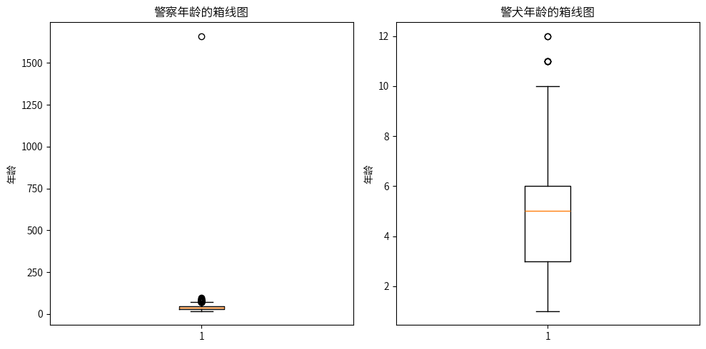
警察年龄这里存在异常值,直接进行删除处理,警犬是可能年龄超过10岁的,因此不处理。
# 将年龄超过100的值替换为NaN
police_data['Age'] = police_data['Age'].apply(lambda x: np.nan if x > 100 else x)
plt.figure(figsize=(5, 5))
# 去除 Age 列中的 NaN 值
police_age_data = police_data['Age'].dropna()
plt.boxplot(police_age_data)  # 绘制箱线图
plt.title("处理后的警察年龄的箱线图")
plt.ylabel("年龄")

plt.tight_layout()
plt.show()
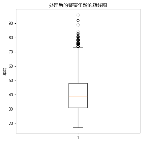
发现还是有特别高龄的警察,这里查看一下。
police_data[police_data['Age'] > 80]
| Rank | Name | Age | End_Of_Watch | Day_Of_Week | Cause | State | Tour | Badge | Weapon | Offender | Summary | |
|---|---|---|---|---|---|---|---|---|---|---|---|---|
| 30 | Town Sergeant | John Smith | 83.0 | 1832-06-21 | Thursday | Assault | Rhode Island | 40 years | NaN | Edged weapon; Axe | Executed | Town Sergeant John Smith was killed as he attempted to arrest a man who was wanted by Connecticut authorities for being a debtor. The Connecticut authorities had tracked the man into Rhode Island, where he had taunted and threatened them with a weapon. Rhode Island authorities swore out a warrant for the man on the charge that he threatened the officers, and Town Sergeant Smith and a small posse went to enforce the warrant. When Town Sergeant Smith approached the wanted man, however, the man attacked him with an ax. The man struck Town Sergeant Smith between the shoulder blades, killing him, and then struck him again in the back of the neck.The assailant then attacked the posse and fled the scene. He was later arrested at the house of a local resident after he bragged about his crime.The assailant was tried and convicted of killing Town Sergeant Smith. He was sentenced to death and hanged on December 27, 1833.Town Sergeant Smith was around 83 years old at the time of his death. He had served as the Town Sergeant of Foster for over 40 years, and also acted as a deputy sheriff. He was survived by his wife and two children. |
| 1885 | Centre Keeper | Jacob Grandine Van Houten | 81.0 | 1896-04-14 | Tuesday | Assault | New Jersey | 40 years | NaN | Person | NaN | Centre Keeper Jacob Van Houten succumbed to injuries sustained one year earlier when he was assaulted by an inmate in the Center Rotunda at the New Jersey State Prison in Trenton.Keeper Van Houten was conducting a disciplinary hearing for the inmate when the man attacked him, knocking him down and fracturing his hip. His condition continued to deteriorate and he eventually died as a result the following year.Centre Keeper Van Houten had served with the New Jersey Department of Corrections for 40 years and was the agency's oldest serving officer at the time of his assault. He was survived by his wife. |
| 2265 | Sheriff | James T. Cooley | 89.0 | 1900-03-03 | Saturday | Assault | Alabama | NaN | NaN | Blunt object; Bat | Died in mental institution | Sheriff James Cooley was beaten to death by an insane prisoner in the Chilton County Jail.The 22-year-old suspect, who had been showing signs of insanity for several months, was placed in the county jail until the papers necessary for his commitment to the insane asylum could be secured. There was only one other prisoner in the jail, so before leaving for the night, the jailer left the partition doors unlocked so both prisoners could enjoy the same stove. During the night, the suspect beat the other prisoner to death with a wooden bat and then lay in wait for the jailer. When Sheriff Cooley opened the jail door about daylight, the suspect crushed his skull and escaped. He was recaptured later that day.The suspect was committed at the Bryce State Mental Hospital in Tuscaloosa, where he died on July 28, 1943. |
| 3376 | Deputy Dispensary Constable | John Dozier Altman | 81.0 | 1909-07-09 | Friday | Gunfire | South Carolina | 1 day | NaN | Handgun | Sentenced to 20 years | Deputy Dispensary Constable John Altman and Dispensary Constable Pinkney Fishburne were shot and killed in Ravenel, South Carolina, while attempting to stop a man from taking a keg of contraband whiskey from the town's railroad station.Constable Fishburne stopped the man as he tried to leave the depot in a horse and buggy. When told he had to turn over the whiskey, the man opened fire, striking Constable Fishburne in the chest. The subject then shot and mortally wounded Deputy Constable Altman, whom Constable Fishburne had deputized to assist him.The subject fled the scene but was arrested a short time later. Constable Fishburne died of his wound approximately one hour later. Deputy Constable Altman was transported to a hospital in Charleston where he died three days later.The man who murdered both officers was convicted of manslaughter and sentenced to 20 years in prison.Deputy Constable Altman was survived by several adult children. |
| 10857 | Chief of Police | Taylor Gray Walker | 81.0 | 1939-09-10 | Sunday | Struck by vehicle | Kentucky | 23 years | NaN | NaN | NaN | Chief Taylor Walker succumbed to injuries sustained 8 days earlier when he was struck by a vehicle, while crossing the street at the town square when he was on duty.\rChief Walker had served as the Adairville police chief for 23 years. He was single and was survived by his nephew. |
| 12339 | Chief of Police | Franklin Pierce Culp | 84.0 | 1950-04-23 | Sunday | Gunfire | Ohio | NaN | NaN | Rifle; Machine gun | The Dillinger Gang | Chief Culp succumbed to gunshot wounds sustained on May 3, 1934, when he and another officer responded to a bank robbery call at the First National Bank at the intersection of Main Street and Tiffin Street. The bank was being robbed by members of the Dillinger Gang.As the officers attempted to take cover behind an elevator one of the suspects opened fire with a machine gun, striking Chief Culp in the chest. The suspects took several hostages, completed the bank robbery, and then fled the scene. |
| 14133 | Police Officer | Carlos S. Stuteville | 96.0 | 1964-08-22 | Saturday | Gunfire | Florida | 15 years | 96 | Officer's handgun | Deported | Police Officer Carlos Stuteville was shot and killed at Miami International Airport. He and an airport security guard were escorting a mentally ill sailor to an airplane for deportation to his native Jamaica. The man began to struggle with Officer Stuteville and gained control of his .38 caliber service revolver. The man shot and killed the security guard before turning and shooting Officer Stuteville, mortally wounding him. The suspect was found not guilty by reason of insanity for Officer Stuteville's murder and subsequently deported to Jamaica.Officer Stuteville had served with the Metro-Dade Police Department for over 15 years. He is survived by his wife and children. |
| 23082 | Sergeant | Harold J. Collins | 92.0 | 2012-05-31 | Thursday | Duty related illness | Massachusetts | 29 years, 3 months | NaN | NaN | NaN | Sergeant Harold Collins contracted poliomyelitis while administering mouth-to-mouth resuscitation of a seven-year-old drowning victim on November 7th, 1955.He responded to a call of the child being found face down and unresponsive in Lee Pool, in modern-day Lederman Park in Boston. He immediately began mouth-to-mouth resuscitation and was able to revive the child.During her hospital stay, the girl was determined to be a carrier of all three strains of the poliovirus. Sergeant Collins contracted the virus and suffered the effects of the disease over the years, and retired from active duty in 1979. Sergeant Collins was struck with the post-polio syndrome in 2004 and died of its effects on May 31st, 2012. Sergeant Collins was a U.S. Navy WWII veteran and served with the Metropolitan Police Department for 29 years. He is survived by his wife, three children, sister, and four grandchildren. |
| 23118 | Chief of Police | Herbert D. Proffitt | 82.0 | 2012-08-28 | Tuesday | Gunfire | Kentucky | 55 years | NaN | Handgun | Apprehended | Chief of Police (Ret) Herbert Proffitt was shot and killed from ambush in the driveway of his home by a man whom he had arrested multiple times over the past 40 years. He was walking down his driveway to check his mail when the subject drove up and opened fire, killing him.The 81-year-old suspect fled the scene but was arrested several hours later.It was later determined that Chief Proffitt had first arrested the man for domestic violence in the 1970s. The conviction resulted in the man spending several years in the state penitentiary. Chief Proffitt arrested the man several more times after his release from prison. When he was arrested for Chief Proffitt's murder, he had copies of the original citations in his possession.Chief Proffitt was a U.S. Army veteran of the Korean War. He had served in law enforcement for 55 years, including as chief of the Tompkinsville Police Department and sheriff of Monroe County. He returned to work as a bailiff with the Monroe County Sheriff's Office after retiring the first time in 2000. He retired again in 2009 at the age of 79. |
| 23894 | Corporal | Robert Lee Walker | 89.0 | 2017-05-02 | Tuesday | Duty related illness | Pennsylvania | 17 years | 136 | Toxic chemicals | Sentenced to 2 years | Corporal Robert Walker died as a result of health complications due to his assignment at the Wade Dump Fire.During the response, Corporal Walker was assigned to the front gate of the property for eight hours and entered a smokey office. He was also assigned to patrol the area. He was diagnosed with aplastic anemia in 1982 and had to retire from the Chester Police Department on medical disability. He died as a result of complications due to his diagnosis on May 2nd, 2017.Corporal Walker was a U.S Army veteran and had served with the Chester Police Department for 17 years. He is survived by his wife, and two children. |
| 24204 | Constable | Willie Houston "Hoot" West | 81.0 | 2019-05-09 | Thursday | Automobile crash | Mississippi | 52 years | NaN | NaN | NaN | Constable Hoot West succumbed to injuries sustained three days earlier when his vehicle left the roadway and struck a tree on Harrison Road.He was serving civil papers when the crash occurred just before 8:00 am on May 6th, 2019. He was transported to North Mississippi Medical Center where he succumbed to his injuries on May 9th.Constable West had served as the elected constable of Lowndes County’s District 1 since 1971 and was serving his 13th consecutive term. He had previously served with the Columbus Police Department and Lowndes County Sheriff’s Office. He had a total of 52 years of law enforcement service and was a founding member and first president of the Mississippi Constables Association.He is survived by his son, two daughters, five grandchildren, five great-grandchildren, mother, brother, and two sisters. |
Carlos S. Stuteville 的应该是徽章编号弄成年龄了,因此将其也设置为Nan,其他的高龄警员看下来虽然觉得有点奇怪,但是没那么严重的矛盾。
# 将年龄为96的值替换为 NaN
police_data.loc[police_data['Age'] == 96, 'Age'] = np.nan
police_data = police_data.drop(columns=["Name", "Badge","Tour", "Weapon", "Offender", "Summary"])
dog_data = dog_data.drop(columns=["Name", "Tour", "Weapon", "Offender", "Summary"])
# 将 End_Of_Watch 列转换为日期时间格式
police_data['End_Of_Watch'] = pd.to_datetime(police_data['End_Of_Watch'], errors='coerce')
dog_data['End_Of_Watch'] = pd.to_datetime(dog_data['End_Of_Watch'], errors='coerce')
5.描述性分析
5.1警察数据
print('警察数据描述性结论:')
police_data.describe(include='all')
警察数据描述性结论:
| Rank | Age | End_Of_Watch | Day_Of_Week | Cause | State | |
|---|---|---|---|---|---|---|
| count | 25638 | 22957.000000 | 25638 | 25638 | 25638 | 25638 |
| unique | 620 | NaN | NaN | 7 | 36 | 58 |
| top | Patrolman | NaN | NaN | Saturday | Gunfire | Texas |
| freq | 3841 | NaN | NaN | 4004 | 12870 | 2183 |
| mean | NaN | 40.219802 | 1955-03-26 05:59:54.945003456 | NaN | NaN | NaN |
| min | NaN | 17.000000 | 1791-01-03 00:00:00 | NaN | NaN | NaN |
| 25% | NaN | 31.000000 | 1923-12-12 12:00:00 | NaN | NaN | NaN |
| 50% | NaN | 39.000000 | 1954-01-21 00:00:00 | NaN | NaN | NaN |
| 75% | NaN | 48.000000 | 1990-01-16 12:00:00 | NaN | NaN | NaN |
| max | NaN | 92.000000 | 2022-12-04 00:00:00 | NaN | NaN | NaN |
| std | NaN | 11.621662 | NaN | NaN | NaN | NaN |
- 职级 (Rank):数据集中共有 25638 条记录,涵盖 620 种不同的警察职级,最常见的职级是 巡警 (Patrolman),出现了 3841 次。
- 年龄 (Age):数据集中有效年龄记录数为 22957 条,最小年龄为 17 岁,最大年龄为 92 岁,平均年龄为 40.22 岁,年龄集中分布在 31 岁到 48 岁之间,中位数为 39 岁,标准差为 11.62 岁,说明存在一定的年龄分布差异。
- 殉职日期 (End_Of_Watch):该数据从1791年1月3日到2022年12月4日。
- 殉职星期 (Day_Of_Week):数据覆盖了 7 个星期几,殉职事件最常发生在 星期六 (Saturday),共记录 4004 次。
- 死亡原因 (Cause):数据集中记录了 36 种不同的死亡原因,枪击 (Gunfire) 是最常见的死亡原因,共计 12870 次,占大部分记录,说明枪击是警察殉职的主要威胁。
- 州 (State):数据涉及 58 个不同州,殉职事件最多的州是 德克萨斯州 (Texas),共发生 2183 次。
# 前五名分析
top_police_rank = police_data['Rank'].value_counts().head(5)
top_police_cause = police_data['Cause'].value_counts().head(5)
top_police_state = police_data['State'].value_counts().head(5)

# 统计 Day_Of_Week 的频次
police_day_of_week_counts = police_data['Day_Of_Week'].value_counts().reindex(['Monday', 'Tuesday', 'Wednesday', 'Thursday', 'Friday', 'Saturday', 'Sunday'])

# 时间趋势分析
police_end_of_watch_counts = police_data['End_Of_Watch'].value_counts().sort_index()

fig = plt.figure(figsize=(20, 15))

# Rank 前五
plt.subplot(3, 3, 1)
ax1 = sns.barplot(x=top_police_rank.index, y=top_police_rank.values, palette='cool', hue=top_police_rank.index, dodge=False, edgecolor='black', legend=False)
plt.title('殉职职级分布(前五)')
plt.xlabel('殉职职级')
plt.ylabel('殉职记录数量')
for p in ax1.patches:
    ax1.annotate(f'{int(p.get_height())}',
                 (p.get_x() + p.get_width() / 2., p.get_height()),
                 ha='center', va='center', fontsize=10, color='black', xytext=(0, 5),
                 textcoords='offset points')

# Cause 前五
plt.subplot(3, 3, 2)
ax2 = sns.barplot(x=top_police_cause.index, y=top_police_cause.values, palette='Greens_d', hue=top_police_cause.index, dodge=False, edgecolor='black', legend=False)
plt.title('警察死亡原因分布(前五)')
plt.xlabel('死亡原因类别')
plt.ylabel('记录数量')
for p in ax2.patches:
    ax2.annotate(f'{int(p.get_height())}',
                 (p.get_x() + p.get_width() / 2., p.get_height()),
                 ha='center', va='center', fontsize=10, color='black', xytext=(0, 5),
                 textcoords='offset points')

# State 前五
plt.subplot(3, 3, 3)
ax3 = sns.barplot(x=top_police_state.index, y=top_police_state.values, palette='Purples_d', hue=top_police_state.index, dodge=False, edgecolor='black', legend=False)
plt.title('殉职事件最多的州(前五)')
plt.xlabel('州名')
plt.ylabel('殉职记录数量')
for p in ax3.patches:
    ax3.annotate(f'{int(p.get_height())}',
                 (p.get_x() + p.get_width() / 2., p.get_height()),
                 ha='center', va='center', fontsize=10, color='black', xytext=(0, 5),
                 textcoords='offset points')

# 年龄直方图
plt.subplot(3, 3, 4)
sns.histplot(police_age_data, kde=True, bins=20, color='orange', edgecolor='black')
plt.title('警察年龄分布及核密度曲线')
plt.xlabel('年龄(岁)')
plt.ylabel('殉职记录数量')

plt.subplot(3, 3, 5)
ax5 = sns.barplot(x=police_day_of_week_counts.index, y=police_day_of_week_counts.values, palette='Oranges', hue=police_day_of_week_counts.index, dodge=False, edgecolor='black', legend=False)
plt.title('殉职事件星期分布')
plt.xlabel('星期')
plt.ylabel('殉职记录数量')
for p in ax5.patches:
    ax5.annotate(f'{int(p.get_height())}',
                 (p.get_x() + p.get_width() / 2., p.get_height()),
                 ha='center', va='center', fontsize=10, color='black', xytext=(0, 5),
                 textcoords='offset points')

# 筛选近五年的数据
police_recent_five_years = police_data[police_data['End_Of_Watch'].dt.year >= (police_data['End_Of_Watch'].dt.year.max() - 4)]

# 按年份统计事件数量
police_recent_year_counts = police_recent_five_years['End_Of_Watch'].dt.year.value_counts().sort_index()

# 绘制折线图
plt.subplot(3, 3, 6)
plt.plot(police_recent_year_counts.index, police_recent_year_counts.values, marker='o', linestyle='-', color='blue')
plt.title('近五年殉职事件数量趋势')
plt.xlabel('年份')
plt.ylabel('殉职事件数量')
plt.grid(axis='y', linestyle='--', alpha=0.7)
plt.gca().xaxis.set_major_locator(mticker.MaxNLocator(integer=True))
# 添加数据标注
for x, y in zip(police_recent_year_counts.index, police_recent_year_counts.values):
    plt.text(x, y + 2, f'{y}', ha='center', va='bottom', fontsize=10, color='black')

plt.subplot(3, 3, (7,9))
police_bins = list(range(police_data['End_Of_Watch'].dt.year.min() // 10 * 10, police_data['End_Of_Watch'].dt.year.max() + 10, 10))
police_labels = [f"{police_bins[i]}-{police_bins[i+1]-1}" for i in range(len(police_bins) - 1)]
police_grouped_end_of_watch = pd.cut(police_data['End_Of_Watch'].dt.year, bins=police_bins, labels=police_labels, right=False).value_counts().sort_index()
plt.plot(police_grouped_end_of_watch.index, police_grouped_end_of_watch.values, marker='o', linestyle='-', color='blue')
plt.title('殉职日期分布趋势(按 10 年分组)')
plt.xlabel('年份分组')
plt.ylabel('殉职事件数量')
plt.grid(axis='y', linestyle='--', alpha=0.7)
for x, y in zip(police_grouped_end_of_watch.index, police_grouped_end_of_watch.values):
    plt.text(x, y + 2, f'{y}', ha='center', va='bottom', fontsize=10, color='black')

plt.tight_layout()
plt.show()
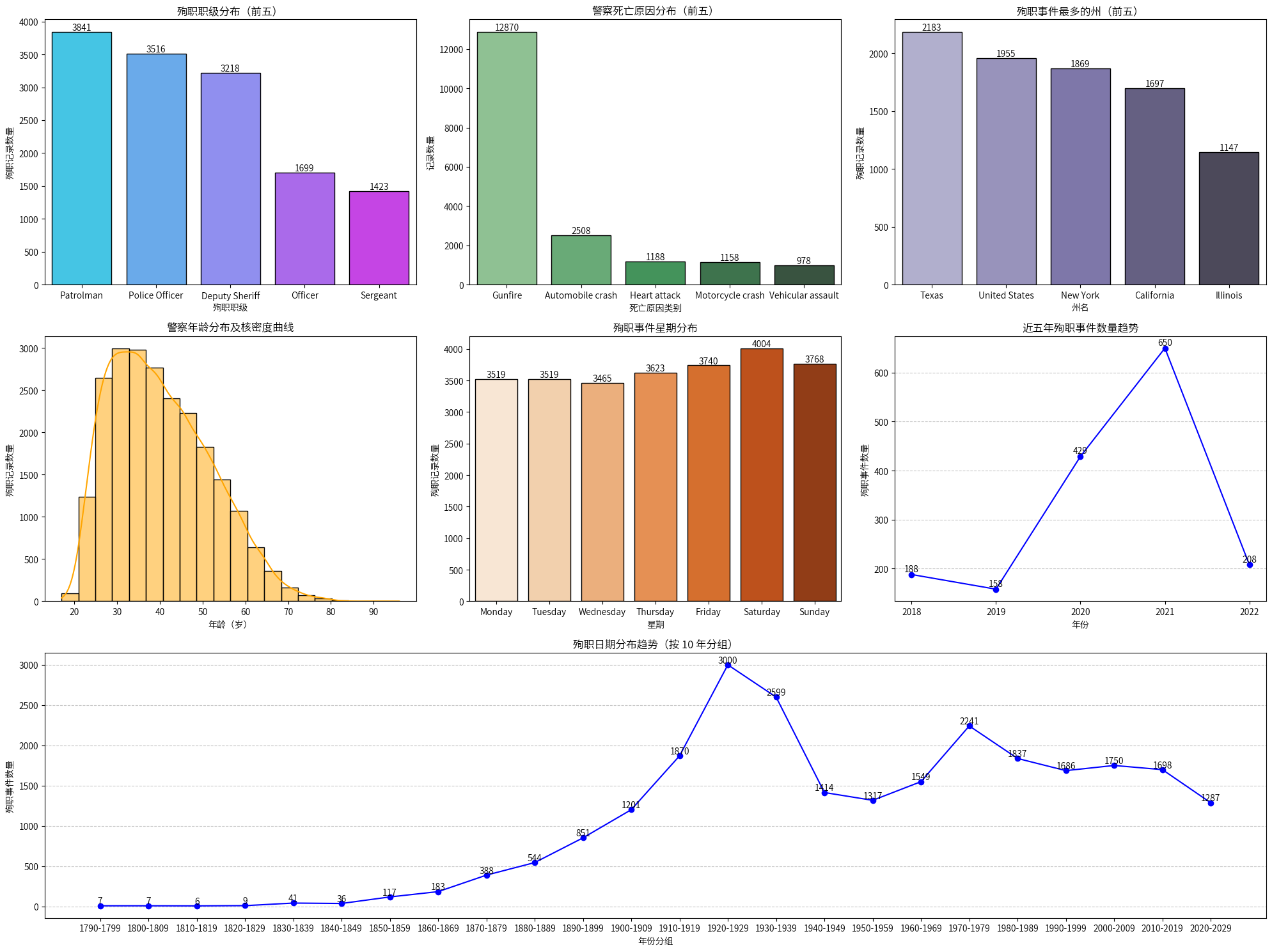
- 在殉职警察中,职级排名前五的依次为巡警、警察官、副警长、警员和警佐,显示出基础执法岗位面临的风险更高,且是殉职的主要人群。
- 枪击是主要的死亡原因,占据了绝大部分记录(共12870次),因此需要为警员提供更有效的防护措施。
- 殉职警察的前五大州依次为德克萨斯州、全美数据(估计是未明确的州,归类为“全美数据”)、纽约州、加利福尼亚州和伊利诺伊州。
- 殉职警察的年龄大多集中在壮年期,这可能与其工作强度和执法职责密切相关。
- 殉职事件发生在周末(尤其是周六)的频率较高,这可能与周末活动增加以及治安工作量上升有关。
- 从2018年到2022年,殉职事件数量波动较大,2021年达到峰值,2022年则显著下降。相关部门应深入研究导致2021年殉职事件激增的原因,并分析出台的政策如何有效降低了2022年的殉职事件。
- 1920至1939年间的殉职记录最多,分别为3000次和2599次,远高于其他时间段。这一现象可能与当时的禁酒令政策有关。“美国禁酒令带来了严重的社会问题,禁酒令根本无法消除人们喝酒的欲望和需求,在正规市场被禁的同时,地下黑市却得到了飞速的发展。非法制造和买卖酒类制品带来的暴利深度挖掘了酒贩子潜力:有人把福特汽车的中间掏空,有人用婴儿车来偷运葡萄酒和白兰地,有人在家里藏酒的地方安装假门。尤其严重的是,在禁酒令实施之前,因为没有财政依据,美国的黑社会波澜不兴,而在实施禁酒令之后,依靠私酒贸易带来的暴利,美国的黑社会开始发展壮大。与此同时,警察也日益腐败,犯罪率不断上升。”
5.2警犬数据
print('警犬数据描述性结论:')
dog_data.describe(include='all')
警犬数据描述性结论:
| Breed | Gender | Age | End_Of_Watch | Day_Of_Week | Cause | State | |
|---|---|---|---|---|---|---|---|
| count | 506 | 506 | 341.000000 | 506 | 506 | 506 | 506 |
| unique | 20 | 3 | NaN | NaN | 7 | 24 | 45 |
| top | German Shepherd | Male | NaN | NaN | Wednesday | Gunfire | California |
| freq | 189 | 415 | NaN | NaN | 88 | 147 | 57 |
| mean | NaN | NaN | 4.891496 | 2006-07-07 04:53:07.351778688 | NaN | NaN | NaN |
| min | NaN | NaN | 1.000000 | 1877-04-12 00:00:00 | NaN | NaN | NaN |
| 25% | NaN | NaN | 3.000000 | 1999-08-19 00:00:00 | NaN | NaN | NaN |
| 50% | NaN | NaN | 5.000000 | 2013-01-03 12:00:00 | NaN | NaN | NaN |
| 75% | NaN | NaN | 6.000000 | 2017-11-27 06:00:00 | NaN | NaN | NaN |
| max | NaN | NaN | 12.000000 | 2022-11-16 00:00:00 | NaN | NaN | NaN |
| std | NaN | NaN | 2.348332 | NaN | NaN | NaN | NaN |
- 品种 (Breed):数据集中共有 506 条记录,涵盖 20 种不同的警犬品种。最常见的警犬品种是 德国牧羊犬 (German Shepherd),出现了 189 次。
- 性别 (Gender):数据中的警犬性别分布为 3 种性别,其中最常见的是 雄性 (Male),出现了 415 次。
- 年龄 (Age):警犬的平均年龄为 4.89 岁,最小年龄为 1 岁,最大年龄为 12 岁,标准差为 2.35 岁,年龄范围集中在 3 岁到 6 岁之间,其中中位数为 5 岁。
- 殉职日期 (End_Of_Watch):该数据从1877年4月12到2022年11月16。
- 殉职星期 (Day_Of_Week):数据涵盖了 7 个星期几,最常见的殉职日是 星期三 (Wednesday),共出现 88 次。
- 死亡原因 (Cause):数据中记录了 24 种不同的死亡原因,最常见的死亡原因是 枪击 (Gunfire),共出现了 147 次,占据大部分记录,显示枪击是警犬殉职的主要原因。
- 州 (State):数据涉及 45 个不同州,发生殉职事件最多的州是 加利福尼亚州 (California),共记录了 57 次。
# 前五名分析
top_dog_breed = dog_data['Breed'].value_counts().head(5)  # 按犬种统计前五
top_dog_cause = dog_data['Cause'].value_counts().head(5)  # 按死亡原因统计前五
top_dog_state = dog_data['State'].value_counts().head(5)  # 按州统计前五

# 统计 Day_Of_Week 的频次(并按照周一到周日排序)
dog_day_of_week_counts = dog_data['Day_Of_Week'].value_counts().reindex(['Monday', 'Tuesday', 'Wednesday', 'Thursday', 'Friday', 'Saturday', 'Sunday'])

# 时间趋势分析
dog_end_of_watch_counts = dog_data['End_Of_Watch'].value_counts().sort_index()

fig = plt.figure(figsize=(20, 15))

# Breed 前五
plt.subplot(3, 3, 1)
ax1 = sns.barplot(x=top_dog_breed.index, y=top_dog_breed.values, palette='cool', hue=top_dog_breed.index, dodge=False, edgecolor='black', legend=False)
plt.title('殉职犬种分布(前五)')
plt.xlabel('殉职犬种')
plt.ylabel('殉职记录数量')
for p in ax1.patches:
    ax1.annotate(f'{int(p.get_height())}',
                 (p.get_x() + p.get_width() / 2., p.get_height()),
                 ha='center', va='center', fontsize=10, color='black', xytext=(0, 5),
                 textcoords='offset points')

# Cause 前五
plt.subplot(3, 3, 2)
ax2 = sns.barplot(x=top_dog_cause.index, y=top_dog_cause.values, palette='Greens_d', hue=top_dog_cause.index, dodge=False, edgecolor='black', legend=False)
plt.title('警犬死亡原因分布(前五)')
plt.xlabel('死亡原因类别')
plt.ylabel('记录数量')
for p in ax2.patches:
    ax2.annotate(f'{int(p.get_height())}',
                 (p.get_x() + p.get_width() / 2., p.get_height()),
                 ha='center', va='center', fontsize=10, color='black', xytext=(0, 5),
                 textcoords='offset points')

# State 前五
plt.subplot(3, 3, 3)
ax3 = sns.barplot(x=top_dog_state.index, y=top_dog_state.values, palette='Purples_d', hue=top_dog_state.index, dodge=False, edgecolor='black', legend=False)
plt.title('殉职事件最多的州(前五)')
plt.xlabel('州名')
plt.ylabel('殉职记录数量')
for p in ax3.patches:
    ax3.annotate(f'{int(p.get_height())}',
                 (p.get_x() + p.get_width() / 2., p.get_height()),
                 ha='center', va='center', fontsize=10, color='black', xytext=(0, 5),
                 textcoords='offset points')

# Gender 饼图
plt.subplot(3, 3, 4)
gender_counts = dog_data['Gender'].value_counts()
plt.pie(gender_counts, labels=gender_counts.index, autopct='%1.1f%%', startangle=90, colors=['#66b3ff', '#99ff99', '#ff6666'])
plt.title('警犬性别分布')

# 年龄分布及核密度曲线
plt.subplot(3, 3, 5)
sns.histplot(dog_data['Age'].dropna(), kde=True, bins=11, color='orange', edgecolor='black')
plt.title('警犬年龄分布及核密度曲线')
plt.xlabel('年龄(岁)')
plt.ylabel('殉职记录数量')

# Day_Of_Week 分布
plt.subplot(3, 3, 6)
ax6 = sns.barplot(x=dog_day_of_week_counts.index, y=dog_day_of_week_counts.values, palette='Oranges', hue=dog_day_of_week_counts.index, dodge=False, edgecolor='black', legend=False)
plt.title('殉职事件星期分布')
plt.xlabel('星期')
plt.ylabel('殉职记录数量')
for p in ax6.patches:
    ax6.annotate(f'{int(p.get_height())}',
                 (p.get_x() + p.get_width() / 2., p.get_height()),
                 ha='center', va='center', fontsize=10, color='black', xytext=(0, 5),
                 textcoords='offset points')

# 筛选近五年的数据
dog_recent_five_years = dog_data[dog_data['End_Of_Watch'].dt.year >= (dog_data['End_Of_Watch'].dt.year.max() - 4)]

# 按年份统计事件数量
dog_recent_year_counts = dog_recent_five_years['End_Of_Watch'].dt.year.value_counts().sort_index()

# 绘制折线图
plt.subplot(3, 3, 7)
plt.plot(dog_recent_year_counts.index, dog_recent_year_counts.values, marker='o', linestyle='-', color='blue')
plt.title('近五年殉职事件数量趋势')
plt.xlabel('年份')
plt.ylabel('殉职事件数量')
plt.grid(axis='y', linestyle='--', alpha=0.7)
plt.gca().xaxis.set_major_locator(mticker.MaxNLocator(integer=True))
# 添加数据标注
for x, y in zip(dog_recent_year_counts.index, dog_recent_year_counts.values):
    plt.text(x, y + 0.5, f'{y}', ha='center', va='bottom', fontsize=10, color='black')

# 10年为一组,殉职日期分布趋势
plt.subplot(3, 3, (8,9))
dog_bins = list(range(dog_data['End_Of_Watch'].dt.year.min() // 10 * 10, dog_data['End_Of_Watch'].dt.year.max() + 10, 10))
dog_labels = [f"{dog_bins[i]}-{dog_bins[i+1]-1}" for i in range(len(dog_bins) - 1)]
dog_grouped_end_of_watch = pd.cut(dog_data['End_Of_Watch'].dt.year, bins=dog_bins, labels=dog_labels, right=False).value_counts().sort_index()
plt.plot(dog_grouped_end_of_watch.index, dog_grouped_end_of_watch.values, marker='o', linestyle='-', color='blue')
plt.title('殉职日期分布趋势(按 10 年分组)')
plt.xlabel('年份分组')
plt.ylabel('殉职事件数量')
plt.grid(axis='y', linestyle='--', alpha=0.7)
for x, y in zip(dog_grouped_end_of_watch.index, dog_grouped_end_of_watch.values):
    plt.text(x, y + 2, f'{y}', ha='center', va='bottom', fontsize=10, color='black')

plt.tight_layout()
plt.show()
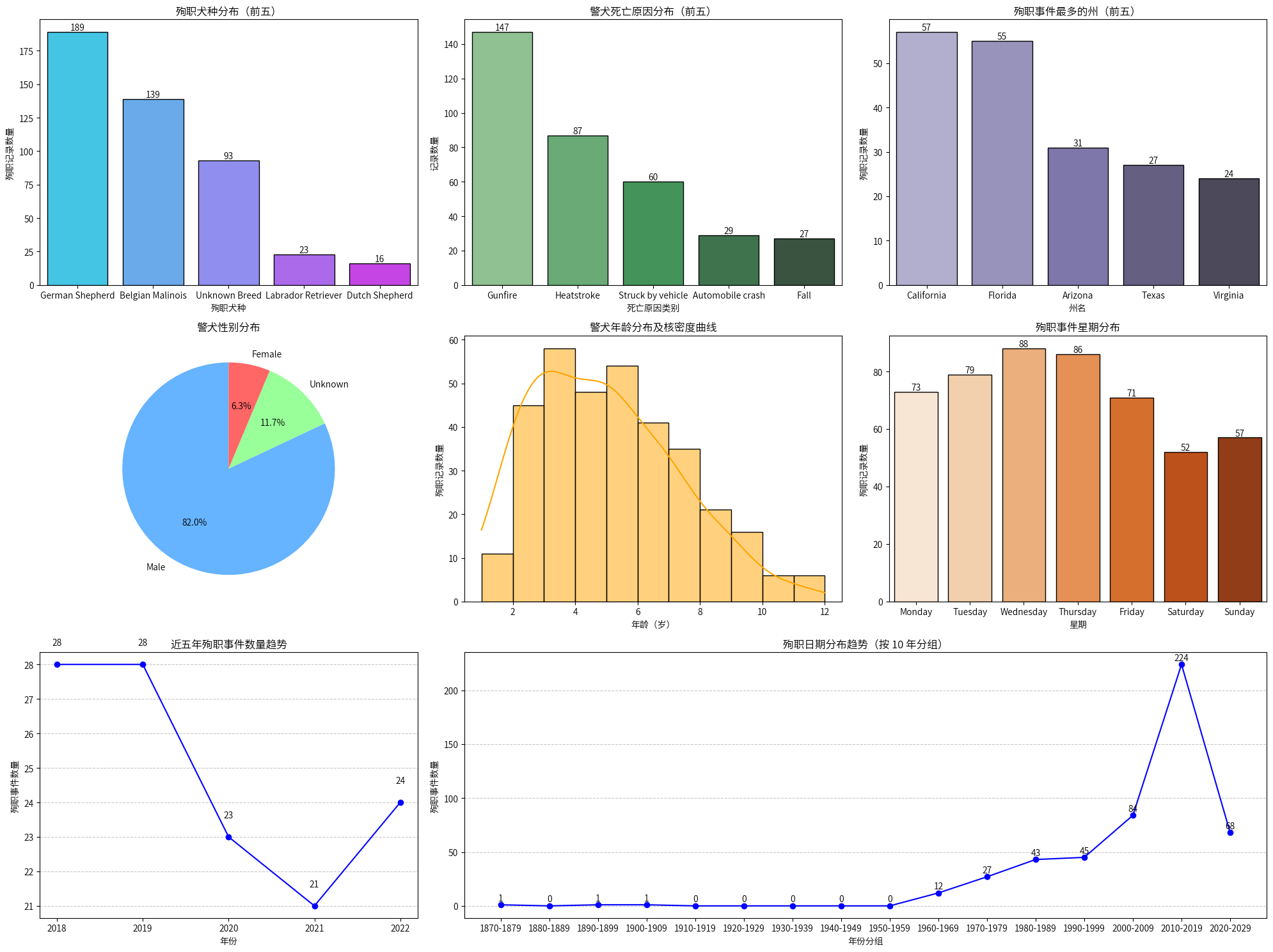
- 德国牧羊犬和马里努阿犬是警犬队伍中最常见的品种,这与它们广泛应用于执法工作中作为搜寻、追捕和保护犬的功能密切相关。因此,在该数据集中,这两类警犬的殉职记录最多。
- 枪击、中暑和汽车事故是警犬死亡的主要原因,这反映了警犬在执行任务过程中面临的多种致命风险。
- 加利福尼亚州和佛罗里达州的警犬死亡记录最多,这可能与这两个州的地理面积、治安状况以及警犬的高使用频率有关。
- 雄性警犬占据了绝大多数的死亡记录,这反映出雄性警犬在警犬队伍中的数量通常较大,从而导致死亡记录的比例较高。
- 殉职警犬的年龄主要集中在壮年期(即工作黄金期),这意味着警犬在执行高强度任务时,正处于其身体和心理最活跃的阶段。
- 与警员相反,警犬的殉职事件主要发生在工作日,尤其是周一至周五,这可能与警犬执行任务的工作时间安排相关。
- 近五年的警犬殉职数量总体保持平稳,但2020-2021年的殉职数量有所下降,这可能与疫情导致的执法活动减少以及公共安全措施的变化有关。
- 美国警犬的使用在近几十年迅速增加,尤其自1960年以后,导致警犬的殉职记录大幅增加,这与警犬在执法中的重要性逐渐提升密切相关。
6.警察分析
6.1常见警察职级随时间变化的趋势分析
# 筛选前五个职级的数据
top_ranks = ['Patrolman', 'Police Officer', 'Deputy Sheriff', 'Officer', 'Sergeant']
filtered_police_data = police_data[police_data['Rank'].isin(top_ranks)]
# 按职级和年份分组,统计每个分组内的事件数量
rank_yearly_counts = pd.crosstab(
    pd.cut(filtered_police_data['End_Of_Watch'].dt.year, bins=police_bins, labels=police_labels, right=False),
    filtered_police_data['Rank']
)
plt.figure(figsize=(20,5))
for rank in top_ranks:
    plt.plot(rank_yearly_counts.index, rank_yearly_counts[rank], marker='o', label=rank)

plt.title('前五大警察职级随时间变化的殉职事件趋势(按 10 年分组)')
plt.xlabel('年份分组')
plt.ylabel('殉职事件数量')
plt.legend(title='警察职级')

plt.grid(axis='y', linestyle='--', alpha=0.7)

plt.tight_layout()
plt.show()
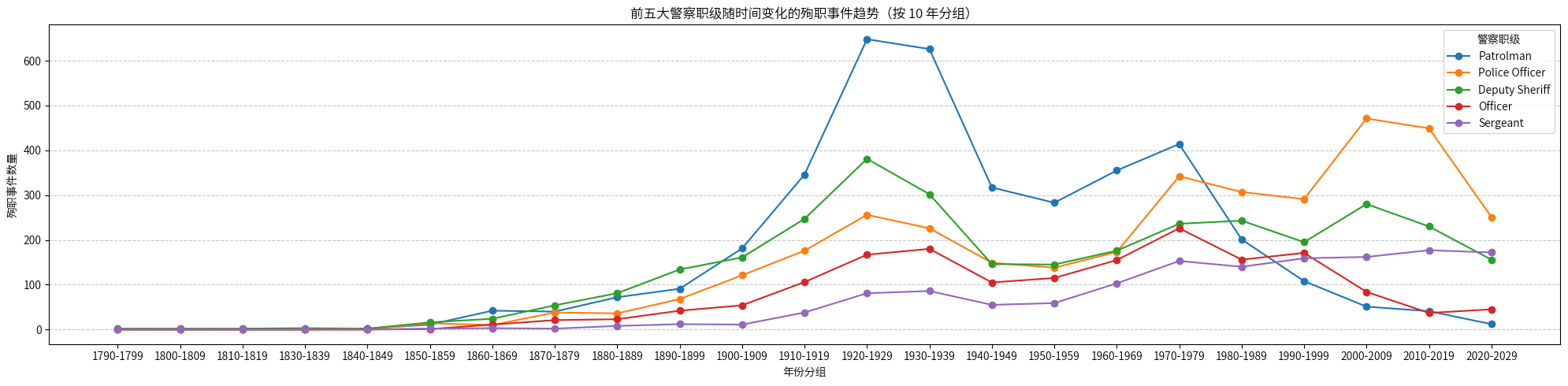
早期,Patrolman(巡警) 的殉职数量最多,但随着时间的推移,Police Officer(警察官)逐渐成为殉职数量最多的职级,而Patrolman的殉职记录则逐渐减少。
6.2警察职级与死亡原因的关联性分析
由于警察职级、死亡原因的唯一值太多了,做卡方检验的话,即使存在轻微的关联,卡方检验的统计量也可能变得非常大,导致p值极小(即便关联可能并无实际意义)。
这里通过claude来辅助完成合并,并且将合并的映射情况保存为json格式,这样只用读取就行。
# 读取映射
with open('/home/mw/project/police_rank_mapping.json', 'r', encoding='utf-8') as f:
    police_rank_mapping = json.load(f)
with open('/home/mw/project/police_cause_mapping.json', 'r', encoding='utf-8') as f:
    police_cause_mapping = json.load(f)
new_police_data = police_data.copy()
new_police_data['Rank'] = new_police_data['Rank'].map(police_rank_mapping)
new_police_data['Cause'] = new_police_data['Cause'].map(police_cause_mapping)
# 创建列联表(交叉表)
rank_cause_table = pd.crosstab(new_police_data['Rank'], new_police_data['Cause'])
# 进行卡方检验
chi2, p, dof, expected = chi2_contingency(rank_cause_table)


print("卡方值 (Chi-Square Statistic):", chi2)
print("p 值 (p-value):", p)
print("自由度 (Degrees of Freedom):", dof)
卡方值 (Chi-Square Statistic): 424.517138126026
p 值 (p-value): 7.995491334533654e-86
自由度 (Degrees of Freedom): 9
通过卡方检验,发现警察职级和死亡原因之间存在统计学显著关联,现在可以使用标准化残差来分析哪一部分数据对检验结果贡献最大。 标准化残差是统计学中的一个重要概念,用于衡量单元格的实际值与期望值之间的差异,以及该差异相对于标准误的显著性。
标准化残差
=
实际值
−
期望值
期望值
\text{标准化残差} = \frac{\text{实际值} - \text{期望值}}{\sqrt{\text{期望值}}}
标准化残差=期望值实际值−期望值
- 实际值:列联表中的观测频数。
- 期望值:基于列联表的总计和卡方检验独立性假设计算得到的频数。
- 期望值 \sqrt{\text{期望值}} 期望值:该单元格频数的标准误。
标准化残差的含义
-
正负性:
- 正残差:实际值大于期望值。
- 负残差:实际值小于期望值。
-
大小:
- ∣ 残差 ∣ > 2 |残差| > 2 ∣残差∣>2:该单元格对卡方检验结果有显著贡献。
- ∣ 残差 ∣ ≤ 2 |残差| ≤ 2 ∣残差∣≤2:该单元格对卡方检验结果贡献较小。
-
解释:
- 如果标准化残差的绝对值较大(例如 ∣ 残差 ∣ > 2 |残差| > 2 ∣残差∣>2),表明该单元格的实际值与期望值的差异显著,说明该分类组合的频数分布与独立性假设存在偏离。
# 将 expected 转换为 DataFrame 并对齐 rank_cause_table
expected_df = pd.DataFrame(expected, index=rank_cause_table.index, columns=rank_cause_table.columns)

# 计算标准化残差
residuals = (rank_cause_table - expected_df) / np.sqrt(expected_df)
print("标准化残差:")
residuals
标准化残差:
| Cause | Accident | Medical | Other | Violent Death |
|---|---|---|---|---|
| Rank | ||||
| Entry-Level Officer | 5.673253 | -7.713774 | 1.123086 | -0.854987 |
| High-Level Officer | -6.037703 | 1.980477 | -1.194960 | 3.549906 |
| Mid-Level Officer | -6.830935 | 14.793201 | -1.577945 | -1.262977 |
| Other | -2.079075 | -0.333201 | 0.311426 | 1.521434 |
1. Entry-Level Officer:
- Accident(5.67):实际值显著高于期望值,说明事故导致的殉职在基层执法者中远高于预期。
- Medical(-7.71):实际值显著低于期望值,说明因疾病导致的殉职在基层执法者中明显少于预期。
2. High-Level Office:
- Accident(-6.04):实际值显著低于期望值,说明高层领导因事故殉职远低于预期。
- Violent Death(3.55):实际值显著高于期望值,说明高层领导因暴力致死的比例高于预期。
3. Mid-Level Officer:
- Accident(-6.83):实际值显著低于期望值,说明中层管理者因事故殉职的比例低于预期。
- Medical(14.79):实际值显著高于期望值,说明中层管理者因疾病殉职的比例远高于预期。
4. Other:
- Accident(-2.08):实际值略低于期望值,接近显著贡献。
6.3美国各州与警察死亡原因的关联性分析
同样的,使用claude将地州划分成东北部、中西部、南部、西部、非连续州(阿拉斯加和夏威夷)、领地和属地(不是美国的50个州,但是属于美国管辖的地区)、联邦(United States)。
with open('/home/mw/project/state_mapping.json', 'r', encoding='utf-8') as f:
    state_mapping = json.load(f)
new_police_data['State'] = new_police_data['State'].map(state_mapping)
# 创建列联表(交叉表)
police_state_cause_table = pd.crosstab(new_police_data['State'], new_police_data['Cause'])
# 进行卡方检验
chi2, p, dof, expected = chi2_contingency(police_state_cause_table)


print("卡方值 (Chi-Square Statistic):", chi2)
print("p 值 (p-value):", p)
print("自由度 (Degrees of Freedom):", dof)
卡方值 (Chi-Square Statistic): 878.8477226959677
p 值 (p-value): 5.08336460448517e-175
自由度 (Degrees of Freedom): 18
expected_df = pd.DataFrame(expected, index=police_state_cause_table.index, columns=police_state_cause_table.columns)

# 计算标准化残差
residuals = (police_state_cause_table - expected_df) / np.sqrt(expected_df)
print("标准化残差:")
residuals
标准化残差:
| Cause | Accident | Medical | Other | Violent Death |
|---|---|---|---|---|
| State | ||||
| Federal | 1.855777 | 0.430653 | 2.408698 | -1.902277 |
| Midwest | -0.838391 | -5.870027 | -0.600757 | 3.176411 |
| Non-Contiguous | 1.470901 | -1.866936 | -0.742280 | -0.090417 |
| Northeast | 4.962165 | 19.744999 | 4.944585 | -12.695600 |
| South | -5.531225 | -3.927897 | -4.238889 | 6.256764 |
| Territories | -3.173505 | -4.857657 | 0.542622 | 4.153425 |
| West | 4.475709 | -6.220991 | 0.667981 | -0.577501 |
1. Federal:
- Other(2.41):实际值显著高于期望值,说明联邦区域的其他原因殉职高于预期。
2. Midwest:
- Medical(-5.87):实际值显著低于期望值,说明中西部因疾病导致的殉职远低于预期。
- Violent Death(3.18):实际值显著高于期望值,说明中西部因暴力致死的比例高于预期。
3. Non-Contiguous:
- 非连续州所有标准化残差的绝对值均小于 2,因此对结果的贡献均不显著。
4. Northeast:
- Accident(4.96):实际值显著高于期望值,说明东北部因事故导致的殉职远高于预期。
- Medical(19.74):实际值显著高于期望值,说明东北部因疾病导致的殉职远高于预期。
- Other(4.94):实际值显著高于期望值,说明东北部因其他原因的殉职远高于预期。
- Violent Death(-12.70):实际值显著低于期望值,说明东北部因暴力致死的比例远低于预期。
5. South:
- Accident(-5.53):实际值显著低于期望值,说明南部因事故导致的殉职比例远低于预期。
- Medical(-3.93):实际值显著低于期望值,说明南部因疾病导致的殉职比例远低于预期。
- Violent Death(6.26):实际值显著高于期望值,说明南部因暴力致死的比例远高于预期。
6. Territories:
- Accident(-3.17):实际值显著低于期望值,说明领地因事故导致的殉职比例远低于预期。
- Medical(-4.86):实际值显著低于期望值,说明领地因疾病导致的殉职比例远低于预期。
- Violent Death(4.15):实际值显著高于期望值,说明领地因暴力致死的比例高于预期。
7. West:
- Accident(4.48):实际值显著高于期望值,说明西部因事故导致的殉职比例远高于预期。
- Medical(-6.22):实际值显著低于期望值,说明西部因疾病导致的殉职比例远低于预期。
7.警犬分析
7.1警犬类型与死亡原因的关联性分析
同样根据claude将警犬品种划分成:牧羊犬类(最传统和常见的警犬品种,智商高,易训练)、工作犬类(体型强壮,保护能力强)、寻回犬类(嗅觉敏锐,适合追踪)、其他类(混血或者未知类型)。
with open('/home/mw/project/dog_breed_mapping.json', 'r', encoding='utf-8') as f:
    dog_breed_mapping = json.load(f)
new_dog_data = dog_data.copy()
new_dog_data['Breed'] = new_dog_data['Breed'].map(dog_breed_mapping)
new_dog_data['Cause'] = new_dog_data['Cause'].map(police_cause_mapping)
breed_cause_table = pd.crosstab(new_dog_data['Breed'], new_dog_data['Cause'])
# 进行卡方检验
chi2, p, dof, expected = chi2_contingency(breed_cause_table)
print("卡方值 (Chi-Square Statistic):", chi2)
print("p 值 (p-value):", p)
print("自由度 (Degrees of Freedom):", dof)
卡方值 (Chi-Square Statistic): 35.523924503195765
p 值 (p-value): 4.814644524331725e-05
自由度 (Degrees of Freedom): 9
breed_cause_table
| Cause | Accident | Medical | Other | Violent Death |
|---|---|---|---|---|
| Breed | ||||
| Hound Dogs | 9 | 22 | 3 | 5 |
| Other/Unknown | 35 | 26 | 6 | 30 |
| Shepherd Dogs | 116 | 74 | 14 | 153 |
| Working Dogs | 4 | 1 | 0 | 8 |
expected_df = pd.DataFrame(expected, index=breed_cause_table.index, columns=breed_cause_table.columns)

# 计算标准化残差
residuals = (breed_cause_table - expected_df) / np.sqrt(expected_df)
print("标准化残差:")
residuals
标准化残差:
| Cause | Accident | Medical | Other | Violent Death |
|---|---|---|---|---|
| Breed | ||||
| Hound Dogs | -1.023906 | 4.066179 | 0.921765 | -2.600310 |
| Other/Unknown | 0.635143 | 0.498566 | 0.757654 | -1.235482 |
| Shepherd Dogs | 0.027191 | -1.371958 | -0.552905 | 1.251370 |
| Working Dogs | -0.103981 | -1.215124 | -0.768706 | 1.321041 |
1. Hound Dogs (猎犬类):
- Medical(4.066):实际值显著高于期望值,说明猎犬因疾病死亡的比例远高于预期。
- Violent Death(-2.600):实际值显著低于期望值,说明猎犬因暴力致死的比例显著低于预期。
2. Other/Unknown (未知或未知混血):
- 所有原因的标准化残差绝对值均小于 2,对结果的贡献均不显著。
3. Shepherd Dogs (牧羊犬类):
- 所有原因的标准化残差绝对值均小于 2,对结果的贡献均不显著。
4. Working Dogs (工作犬类):
- 所有原因的标准化残差绝对值均小于 2,对结果的贡献均不显著。
7.2美国各州与警犬死亡原因的关联性分析
new_dog_data['State'] = new_dog_data['State'].map(state_mapping)
# 创建列联表(交叉表)
dog_state_cause_table = pd.crosstab(new_dog_data['State'], new_dog_data['Cause'])
# 进行卡方检验
chi2, p, dof, expected = chi2_contingency(dog_state_cause_table)


print("卡方值 (Chi-Square Statistic):", chi2)
print("p 值 (p-value):", p)
print("自由度 (Degrees of Freedom):", dof)
卡方值 (Chi-Square Statistic): 38.37577697667609
p 值 (p-value): 0.0007937851122921515
自由度 (Degrees of Freedom): 15
expected_df = pd.DataFrame(expected, index=dog_state_cause_table.index, columns=dog_state_cause_table.columns)

# 计算标准化残差
residuals = (dog_state_cause_table - expected_df) / np.sqrt(expected_df)
print("标准化残差:")
residuals
标准化残差:
| Cause | Accident | Medical | Other | Violent Death |
|---|---|---|---|---|
| State | ||||
| Federal | 0.339262 | 0.177481 | 1.222790 | -0.869810 |
| Midwest | -0.529871 | 0.293599 | -0.519782 | 0.430163 |
| Non-Contiguous | -0.805122 | -0.697256 | -0.301511 | 1.392110 |
| Northeast | 2.821273 | -0.964857 | -0.865768 | -1.519790 |
| South | -1.674170 | 1.724248 | 1.972880 | -0.510328 |
| West | 0.802607 | -1.849658 | -2.008527 | 1.419134 |
1. Federal (联邦):
- 所有原因的标准化残差绝对值均小于 2,对结果的贡献均不显著。
2. Midwest (中西部):
- 所有原因的标准化残差绝对值均小于 2,对结果的贡献均不显著。
3. Non-Contiguous (非连续州):
- 所有原因的标准化残差绝对值均小于 2,对结果的贡献均不显著。
4. Northeast (东北部):
- Accident(2.821):实际值显著高于期望值,说明东北部因事故导致的警犬死亡显著高于预期。
5. South (南部):
- Other(1.973):实际值接近显著高于期望值,说明南部因其他原因导致的警犬死亡略高于预期。
6. West (西部):
- Other(-2.009):实际值显著低于期望值,说明西部因其他原因导致的警犬死亡显著低于预期。
8.总结与建议
8.1总结
基于对1791-2022年间美国警察死亡数据和1877-2022年间警犬死亡数据的全面分析,本项目得出以下主要结论:
1.时间特性分析:
- 警察死亡数据显示1920-1939年间的殉职记录最高,可能与当时的禁酒令政策导致的社会治安恶化有关
- 警犬死亡数据显示自1960年后记录显著增加,反映了警犬在执法中的重要性逐渐提升
- 近五年来,警察殉职数据在2021年达到峰值后显著下降,而警犬殉职数量则相对稳定
2.职级与死因分析:
- 基层执法者更容易因事故殉职,而较少因疾病死亡
- 高层领导较少因事故殉职,但暴力致死比例较高
- 中层管理者因疾病殉职的比例远高于预期,事故致死比例较低
3.地区差异分析:
- 东北部的警察更容易因事故和疾病殉职,但暴力致死比例较低
- 南部和领地的警察较少因事故和疾病殉职,但暴力致死比例较高
- 西部地区的警察和警犬都较容易因事故殉职
4.警犬特征分析:
- 德国牧羊犬是最常见的警犬品种,主要用于执法工作
- 猎犬类警犬较容易因疾病死亡,但较少因暴力致死
- 雄性警犬占据了绝大多数的死亡记录
- 警犬殉职主要发生在工作日,这与警察殉职多发生在周末形成对比
8.2建议
基于以上分析结果,提出以下建议:
-
针对警员保护的建议:
- 加强基层执法人员的安全培训,特别是事故预防方面的教育,因为数据显示基层警员更容易发生事故致死
- 为高层领导配备专业的安保人员,增加保护力度,以降低暴力致死的风险
- 定期进行健康检查,尤其是对中层管理人员,因为数据显示他们因疾病殉职的比例较高
- 在周末增派警力,优化人员配置,因为数据显示周末是警察殉职的高发期
-
区域性安全策略:
- 东北部地区应加强交通安全管理,改善执法环境,降低事故发生率
- 南部和领地应加强警员防护装备配置,增加巡逻密度,以应对较高的暴力风险
- 西部地区需要改善道路条件和执法环境,降低事故发生率
-
警犬管理建议:
- 建立专业的警犬健康管理体系,特别是针对猎犬类警犬的疾病预防
- 优化警犬工作时间安排,避免在极端天气条件下执勤,预防中暑等意外
- 增加母犬在警犬队伍中的比例,平衡性别结构,观察是否能提高整体执行效率
- 根据不同品种的特点分配任务,如将德国牧羊犬主要用于追踪和制服嫌疑人,猎犬类主要用于搜救任务
-
系统性改革建议:
- 建立全国统一的警务人员和警犬伤亡数据库,实时更新和分析数据
- 完善保险体系,为警务人员和警犬提供更全面的保障
- 加强各州之间的经验交流,推广成功的安全防护措施
- 定期评估安全措施的有效性,及时调整和优化保护策略
-
培训与发展建议:
- 开展针对性的训练课程,如为基层警员增加事故预防培训
- 加强心理辅导,帮助警员应对工作压力,预防因压力导致的意外
- 优化警犬训练方案,根据不同品种的特点制定专门的培训计划
- 定期组织应急演练,提高警员和警犬的协同作战能力
这些建议的实施需要警务部门的统筹规划,各级部门的密切配合,以及充足的资金支持。建议分步骤、有计划地推进,优先解决最紧迫的安全问题,逐步建立更完善的警务人员和警犬保护体系。


 被折叠的 条评论
为什么被折叠?
被折叠的 条评论
为什么被折叠?
 到【灌水乐园】发言


