


目录
1.数据集的创建
import numpy as np
import pandas as pd
#数据集的创建
def create_data():
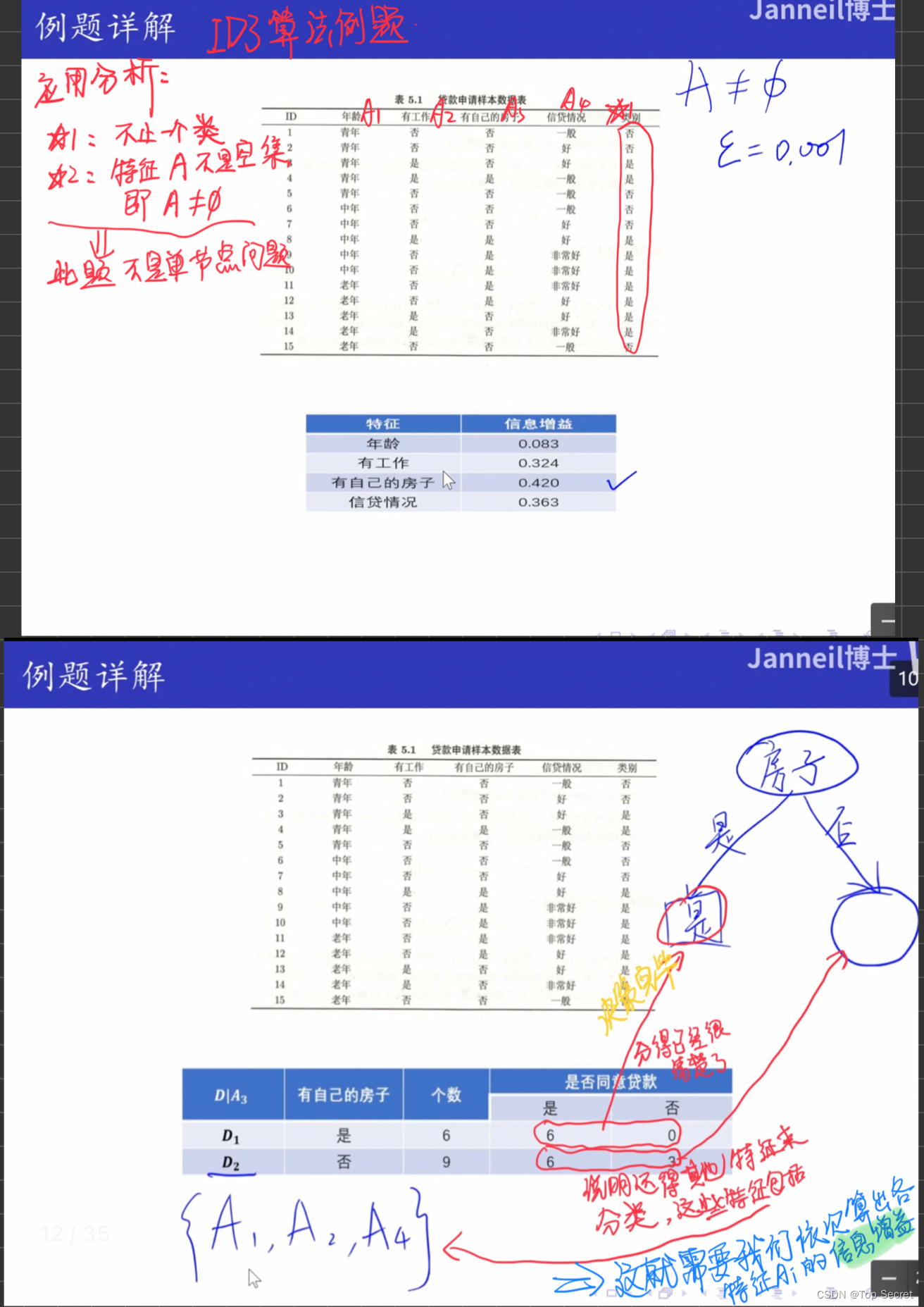
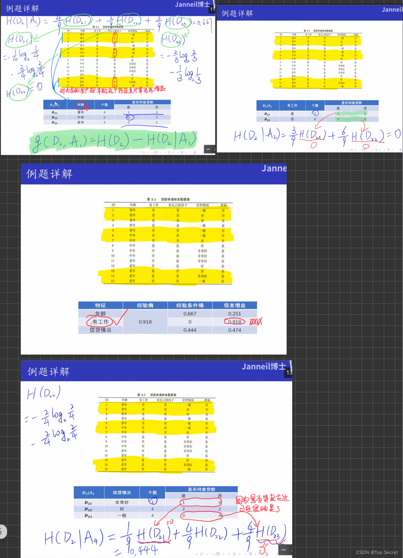
datasets = [['青年', '否', '否', '一般', '否'],
['青年', '否', '否', '好', '否'],
['青年', '是', '否', '好', '是'],
['青年', '是', '是', '一般', '是'],
['青年', '否', '否', '一般', '否'],
['中年', '否', '否', '一般', '否'],
['中年', '否', '否', '好', '否'],
['中年', '是', '是', '好', '是'],
['中年', '否', '是', '非常好', '是'],
['中年', '否', '是', '非常好', '是'],
['老年', '否', '是', '非常好', '是'],
['老年', '否', '是', '好', '是'],
['老年', '是', '否', '好', '是'],
['老年', '是', '否', '非常好', '是'],
['老年', '否', '否', '一般', '否'],
]
labels = [u'年龄', u'有工作', u'有自己的房子', u'信贷情况', u'类别'] #前缀u表示该字符串是unicode编码,防止因为编码问题,导致中文出现乱码
# 返回数据集和每个维度的名称
return datasets, labels
datasets, labels = create_data() #调用数据集创建函数
train_data = pd.DataFrame(datasets, columns=labels) # 创建DataFrame表
print(train_data)
输出:

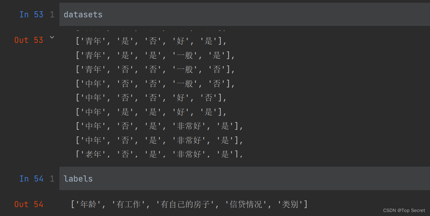
注意:datasets对应的应该就是数据集,而通过pandas的DataFrame创建得就是一个表。
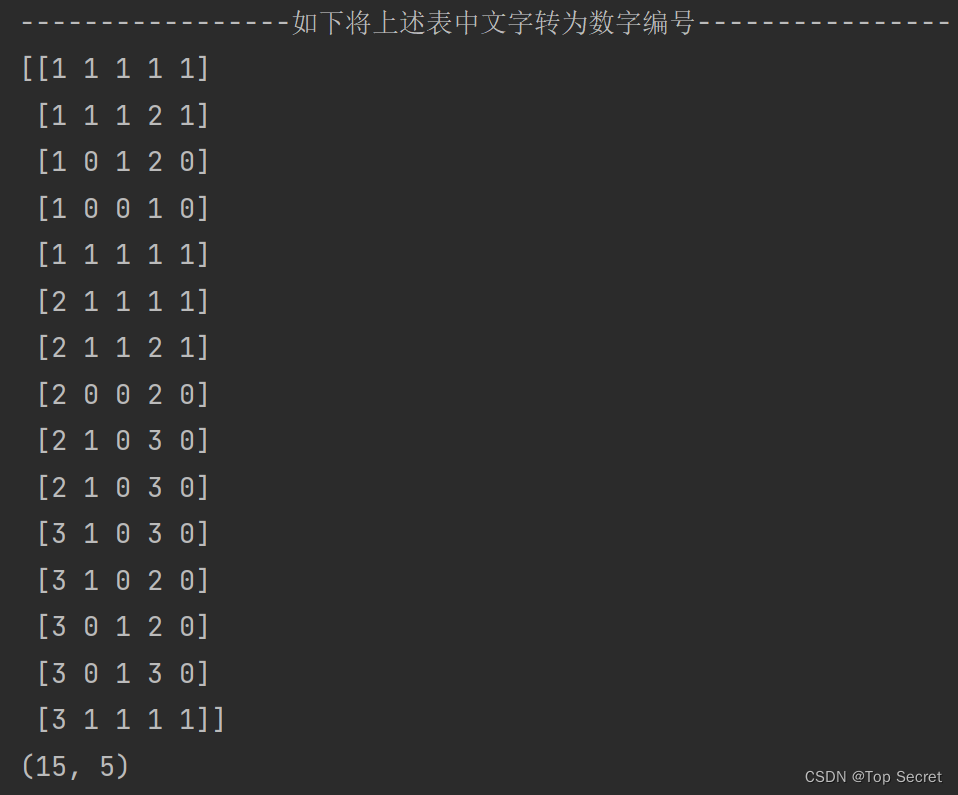
2.将上述表中文字转为数字编号 ,并转为numpy格式
d = {'青年':1, '中年':2, '老年':3, '一般':1, '好':2, '非常好':3, '是':0, '否':1}
data = []  #定义空表用以存放编号后的数据表
for i in range(15):  #表中一共有15组数据
    tmp = []
    t = datasets[i]  #依次打印表中的各组数据,如:t=datasets[1] ---> ['青年', '否', '否', '好', '否']
    for tt in t:            #此处tt读取的分别是键:'青年', '否', '否', '好', '否'
        tmp.append(d[tt])   # 此步接如上,依次为上行代码的键按 d{} 中规则配对
    data.append(tmp)  # 注意:上步中的tmp中只存了一组编码后的数据。而data中依次存入各组数据构成数据表

data = np.array(data) #将表转为numpy的格式
print(data)
print(data.shape)  #查看数据形状
输出:
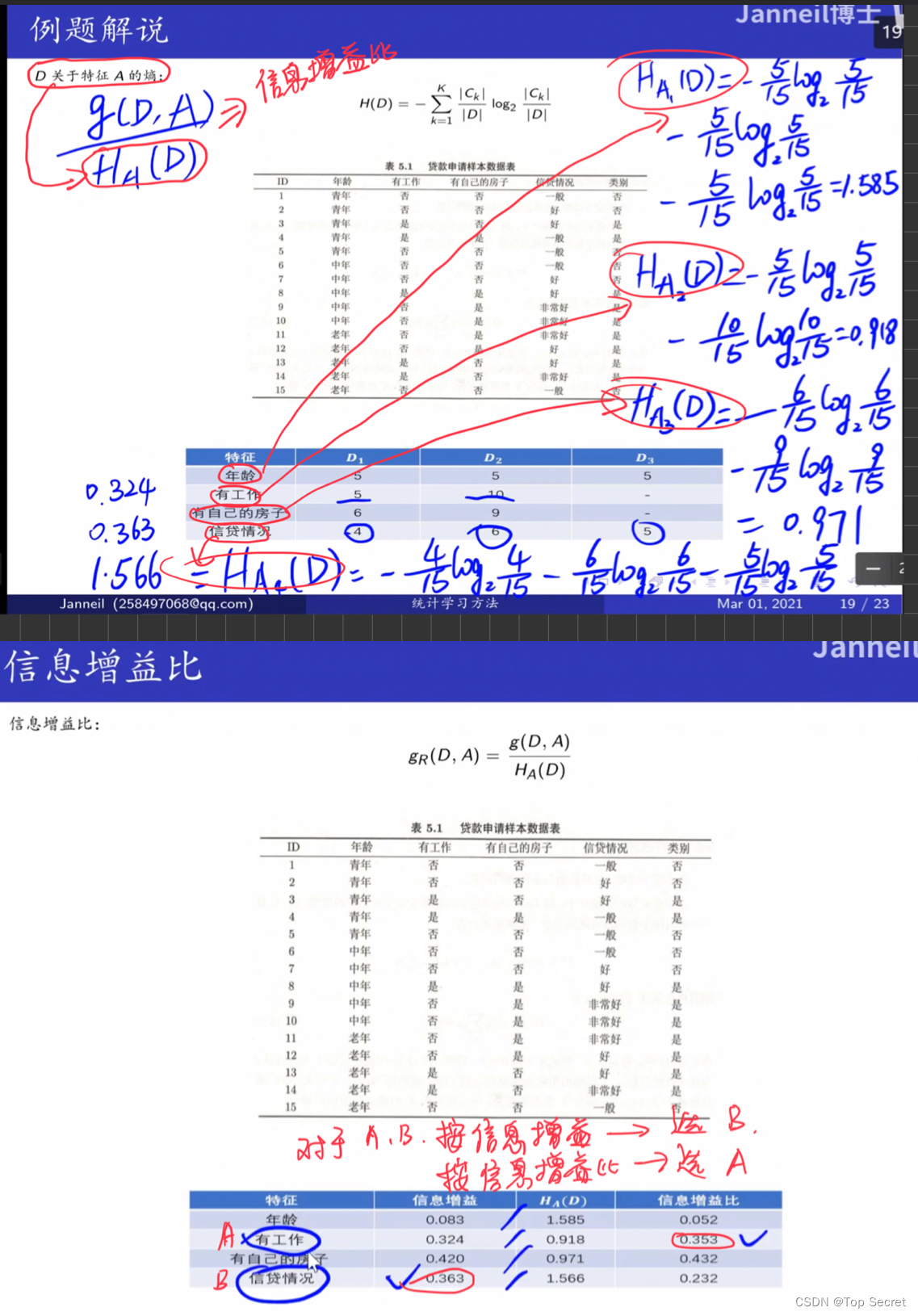
3.熵与条件熵的计算
理论:
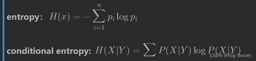
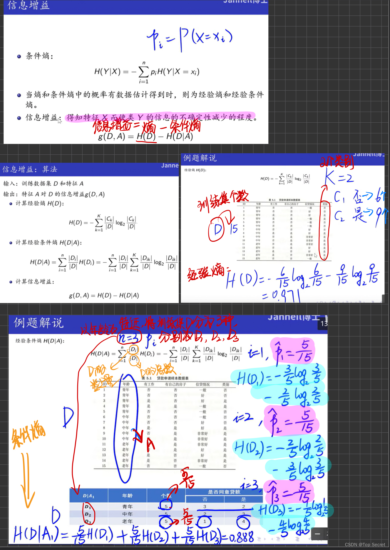
# 熵的计算
def entropy(y):
    N = len(y)
    count = []
    for value in set(y):
        count.append(len(y[y == value]))
    count = np.array(count)
    entro = -np.sum((count / N) * (np.log2(count / N)))
    return entro

# 条件熵的计算
def cond_entropy(X, y, cond):
    N = len(y)
    cond_X = X[:, cond]
    tmp_entro = []
    for val in set(cond_X):
        tmp_y = y[np.where(cond_X == val)]
        tmp_entro.append(len(tmp_y)/N * entropy(tmp_y))
    cond_entro = sum(tmp_entro)
    return cond_entro

#准备好计算熵与条件熵的数据
#data[:,:-1] 依次取每一组数据中除最后一位以外的数
#data[:, -1] 依次取每一组数据中的最后一位
X, y = data[:,:-1], data[:, -1]

Entropy = entropy(y) #计算熵
Cond_entropy = cond_entropy(X, y, 0) #计算条件熵
print("熵:",Entropy)
print("条件熵:",Cond_entropy)
4.计算信息增益与信息增益比
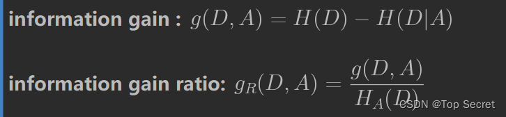
# 信息增益
def info_gain(X, y, cond):
    return entropy(y) - cond_entropy(X, y, cond)
# 信息增益比
def info_gain_ratio(X, y, cond):
    return (entropy(y) - cond_entropy(X, y, cond))/cond_entropy(X, y, cond)

# A1, A2, A3, A4 =》年龄 工作 房子 信贷
# 信息增益
gain_a1 = info_gain(X, y, 0)
print("年龄信息增益:",gain_a1)
gain_a2 = info_gain(X, y, 1)
gain_a3 = info_gain(X, y, 2)
gain_a4 = info_gain(X, y, 3)
print("工作信息增益:",gain_a2)
print("房子信息增益:",gain_a3)
print("信贷信息增益:",gain_a4)
5.特征选择
def best_split(X, y, method='info_gain'):
    """根据method指定的方法使用信息增益或信息增益比来计算各个维度的最大信息增益(比),返回特征的axis"""
    _, M = X.shape
    info_gains = []
    if method == 'info_gain':
        split = info_gain
    elif method == 'info_gain_ratio':
        split = info_gain_ratio
    else:
        print('No such method')
        return
    for i in range(M):
        tmp_gain = split(X, y, i)
        info_gains.append(tmp_gain)
    best_feature = np.argmax(info_gains)

    return best_feature

print(best_split(X,y)) #result--> 2

def majorityCnt(y):
    """当特征使用完时,返回类别数最多的类别"""
    unique, counts = np.unique(y, return_counts=True)
    max_idx = np.argmax(counts)
    return unique[max_idx]

print(majorityCnt(y))
输出:0.
6.完整程序:
import numpy as np
import pandas as pd
# import matplotlib.pyplot as plt
# #matplotlib inline
#
# from sklearn.datasets import load_iris
# from sklearn.model_selection import train_test_split
#
# from collections import Counter
# import math
# from math import log
#
# import pprint

#数据集的创建
def create_data():
    datasets = [['青年', '否', '否', '一般', '否'],
               ['青年', '否', '否', '好', '否'],
               ['青年', '是', '否', '好', '是'],
               ['青年', '是', '是', '一般', '是'],
               ['青年', '否', '否', '一般', '否'],
               ['中年', '否', '否', '一般', '否'],
               ['中年', '否', '否', '好', '否'],
               ['中年', '是', '是', '好', '是'],
               ['中年', '否', '是', '非常好', '是'],
               ['中年', '否', '是', '非常好', '是'],
               ['老年', '否', '是', '非常好', '是'],
               ['老年', '否', '是', '好', '是'],
               ['老年', '是', '否', '好', '是'],
               ['老年', '是', '否', '非常好', '是'],
               ['老年', '否', '否', '一般', '否'],
               ]
    labels = [u'年龄', u'有工作', u'有自己的房子', u'信贷情况', u'类别']  #前缀u表示该字符串是unicode编码,防止因为编码问题,导致中文出现乱码
    # 返回数据集和每个维度的名称
    return datasets, labels

# 熵的计算
def entropy(y):
    N = len(y)
    count = []
    for value in set(y):
        count.append(len(y[y == value]))
    count = np.array(count)
    entro = -np.sum((count / N) * (np.log2(count / N)))
    return entro

# 条件熵的计算
def cond_entropy(X, y, cond):
    N = len(y)
    cond_X = X[:, cond]
    tmp_entro = []
    for val in set(cond_X):
        tmp_y = y[np.where(cond_X == val)]
        tmp_entro.append(len(tmp_y)/N * entropy(tmp_y))
    cond_entro = sum(tmp_entro)
    return cond_entro


datasets, labels = create_data()  #调用数据集创建函数
train_data = pd.DataFrame(datasets, columns=labels)  # 创建DataFrame表

print(train_data)
print("-----------------如下将上述表中文字转为数字编号----------------")

"""
测试:
t = datasets[1]
d = {'青年':1, '中年':2, '老年':3, '一般':1, '好':2, '非常好':3, '是':0, '否':1}
print(t)
['青年', '否', '否', '好', '否']
print(d['青年'])
1
"""

d = {'青年':1, '中年':2, '老年':3, '一般':1, '好':2, '非常好':3, '是':0, '否':1}
data = []  #定义空表用以存放编号后的数据表
for i in range(15):  #表中一共有15组数据
    tmp = []
    t = datasets[i]  #依次打印表中的各组数据,如:t=datasets[1] ---> ['青年', '否', '否', '好', '否']
    for tt in t:            #此处tt读取的分别是键:'青年', '否', '否', '好', '否'
        tmp.append(d[tt])   # 此步接如上,依次为上行代码的键按 d{} 中规则配对
    data.append(tmp)  # 注意:上步中的tmp中只存了一组编码后的数据。而data中依次存入各组数据构成数据表

data = np.array(data) #将表转为numpy的格式
print(data)
print(data.shape)  #查看数据形状

#准备好计算熵与条件熵的数据
#data[:,:-1] 依次取每一组数据中除最后一位以外的数
#data[:, -1] 依次取每一组数据中的最后一位
X, y = data[:,:-1], data[:, -1]

Entropy = entropy(y) #计算熵
Cond_entropy = cond_entropy(X, y, 0) #计算条件熵
print("熵:",Entropy)
print("条件熵:",Cond_entropy)

# 信息增益
def info_gain(X, y, cond):
    return entropy(y) - cond_entropy(X, y, cond)
# 信息增益比
def info_gain_ratio(X, y, cond):
    return (entropy(y) - cond_entropy(X, y, cond))/cond_entropy(X, y, cond)

# A1, A2, A3, A4 =》年龄 工作 房子 信贷
# 信息增益
gain_a1 = info_gain(X, y, 0)
print("年龄信息增益:",gain_a1)
gain_a2 = info_gain(X, y, 1)
gain_a3 = info_gain(X, y, 2)
gain_a4 = info_gain(X, y, 3)
print("工作信息增益:",gain_a2)
print("房子信息增益:",gain_a3)
print("信贷信息增益:",gain_a4)


def best_split(X, y, method='info_gain'):
    """根据method指定的方法使用信息增益或信息增益比来计算各个维度的最大信息增益(比),返回特征的axis"""
    _, M = X.shape
    info_gains = []
    if method == 'info_gain':
        split = info_gain
    elif method == 'info_gain_ratio':
        split = info_gain_ratio
    else:
        print('No such method')
        return
    for i in range(M):
        tmp_gain = split(X, y, i)
        info_gains.append(tmp_gain)
    best_feature = np.argmax(info_gains)

    return best_feature

print(best_split(X,y)) #result--> 2

def majorityCnt(y):
    """当特征使用完时,返回类别数最多的类别"""
    unique, counts = np.unique(y, return_counts=True)
    max_idx = np.argmax(counts)
    return unique[max_idx]

print(majorityCnt(y))
7. ID3算法:
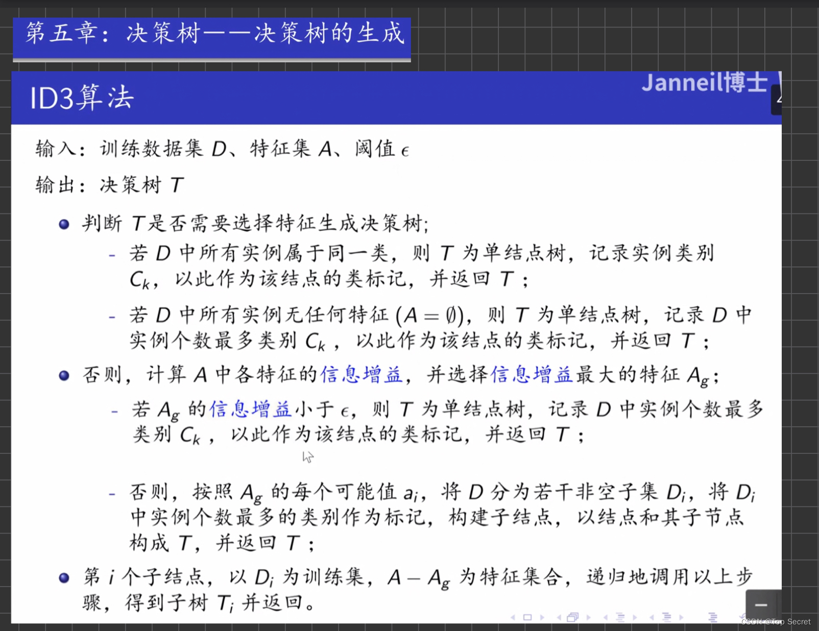
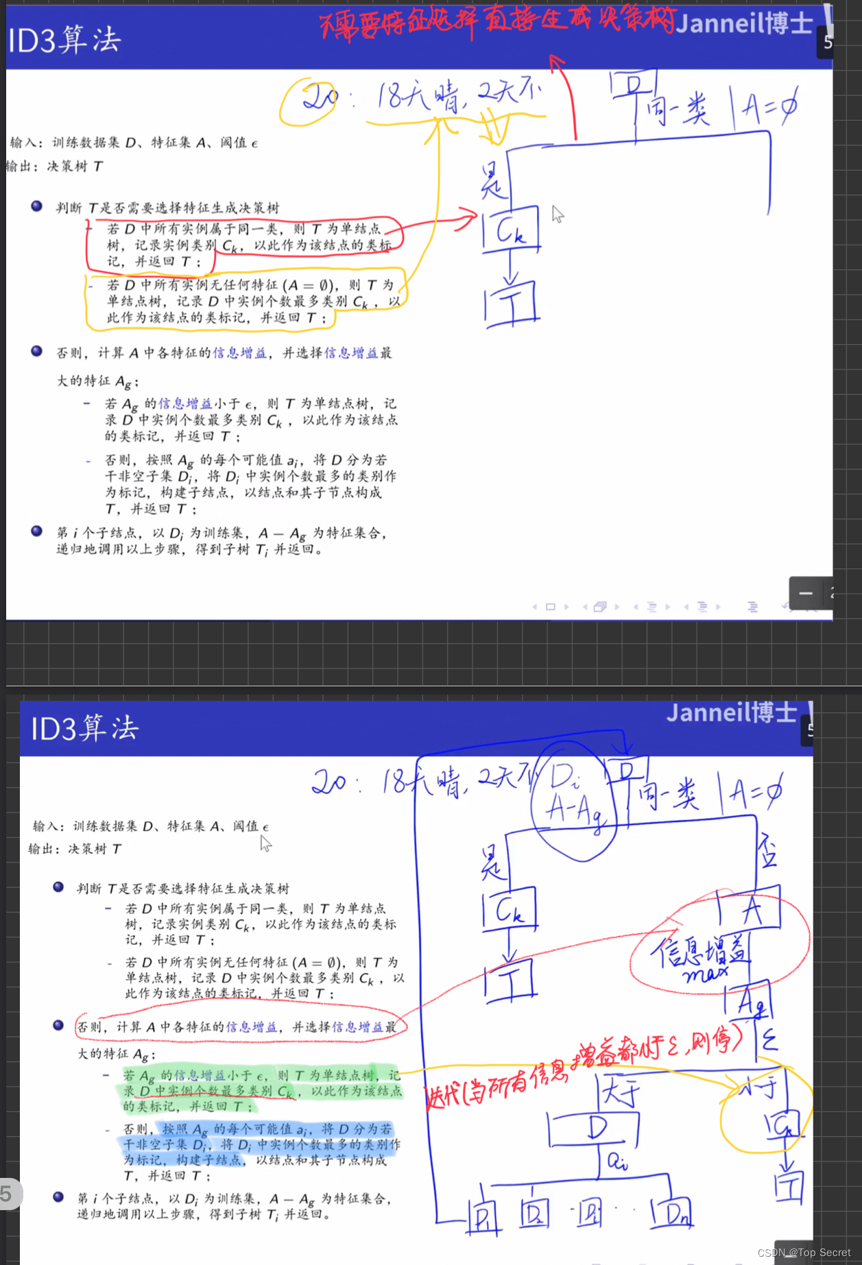
7.1 代码
7.1.1 决策树的生成算法:
class DecisionTreeClassifer:
    """
    决策树生成算法,
    method指定ID3或C4.5,两方法唯一不同在于特征选择方法不同
    info_gain:       信息增益即ID3
    info_gain_ratio: 信息增益比即C4.5


    """

    def __init__(self, threshold, method='info_gain'):
        self.threshold = threshold
        self.method = method

    def fit(self, X, y, labels):
        labels = labels.copy()
        M, N = X.shape
        if len(np.unique(y)) == 1:
            return y[0]

        if N == 1:
            return majorityCnt(y)

        bestSplit = best_split(X, y, method=self.method)
        bestFeaLable = labels[bestSplit]
        Tree = {bestFeaLable: {}}
        del (labels[bestSplit])

        feaVals = np.unique(X[:, bestSplit])
        for val in feaVals:
            idx = np.where(X[:, bestSplit] == val)
            sub_X = X[idx]
            sub_y = y[idx]
            sub_labels = labels
            Tree[bestFeaLable][val] = self.fit(sub_X, sub_y, sub_labels)

        return Tree

My_Tree = DecisionTreeClassifer(threshold=0.1)

print("tree:",My_Tree.fit(X, y, labels))
8.决策树的剪枝
(待补充....)
(学习笔记,侵删。欢迎讨论呢)


 1715
1715


 被折叠的 条评论
为什么被折叠?
被折叠的 条评论
为什么被折叠?
 到【灌水乐园】发言


