电脑销售数据分析

一、数据描述

电商平台在售笔记本产品信息

1. brand：品牌
2. model：型号
3. processor_brand：处理器品牌
4. processor_name：处理器名称
5. processor_gnrtn：intel第几代处理器
6. ram：内存（单位：GB）
7. ssd：固态硬盘（单位：GB）
8. hdd：机械硬盘（单位：GB）
9. os：操作系统
10. graphic_card_gb：独立显卡（0：无独立显卡，>0：有独立显卡，数值为显存容量，单位：GB）
11. weight：重量（Light：轻，Normal：正常，Heavy：重）
12. display_size：屏幕尺寸（单位：英寸）
13. warranty：质保时间（单位：年）
14. touchscreen：是否为触摸屏（0：非触摸屏，1：触摸屏）
15. msoffice：是否赠送office（0：不赠送，1：赠送）
16. latest_price：当前价格
17. old_price：上市价格
18. star_rating：顾客对产品的评级
19. ratings：参与评级的顾客人数（有多少人对该产品进行了评级）
20. reviews：评论数（有多少人对该产品进行评论）

None：缺失值

二、数据分析

import pandas as pd
import numpy as np
import seaborn as sns
import matplotlib.pyplot as plt
plt.rcParams['font.family'] = ['SimHei']
# 正常显示正负号
plt.rcParams['axes.unicode_minus'] = False
data = pd.read_csv(r'D:\桌面\电脑数据分析\Laptop.csv',engine='python')

# 查看数据
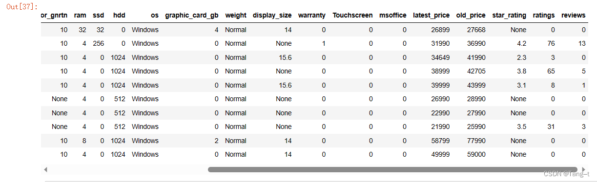
data.head(10)

 输出：

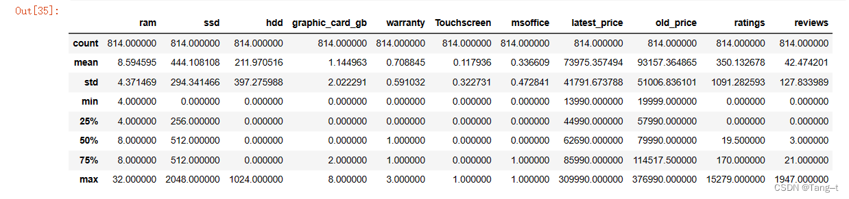
# 数据描述
data.describe()

输出：

data1 = data.replace('None',np.nan)
data1.isnull().sum()
import missingno as msno
msno.bar(data1)

输出：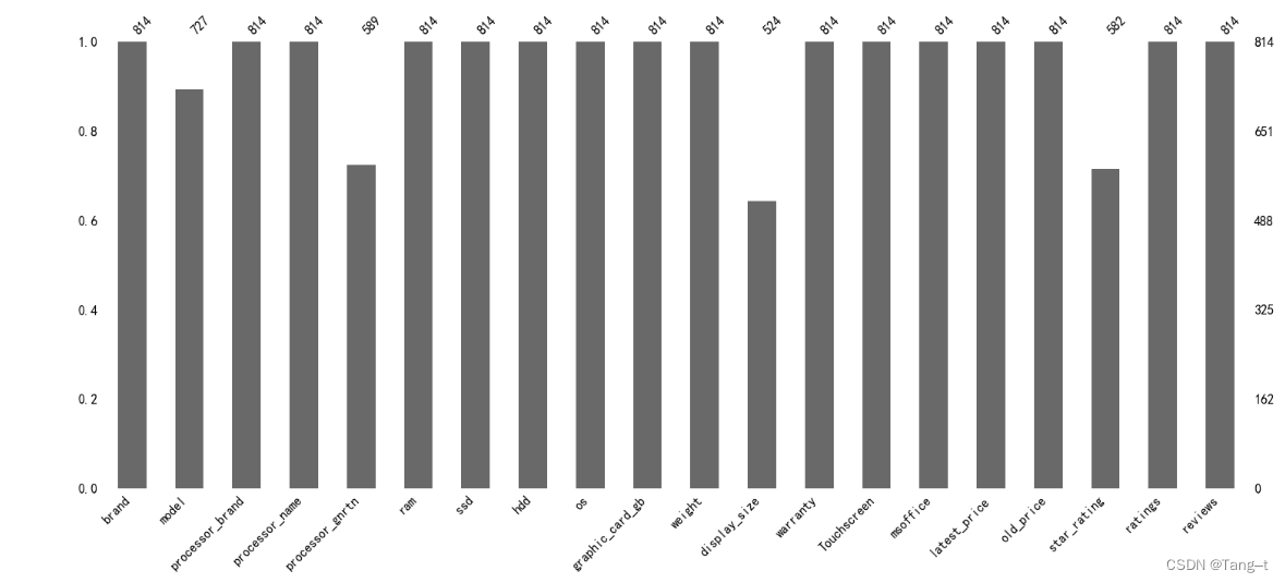

# 计算各变量之间的相关系数
corr = data.corr()
ax = plt.subplots(figsize=(10,10))  # 调整画布大小
sns.heatmap(corr, square=True, annot=True,cmap='cool')  # 画热力图   annot=True 表示显示系数
plt.show()

 输出：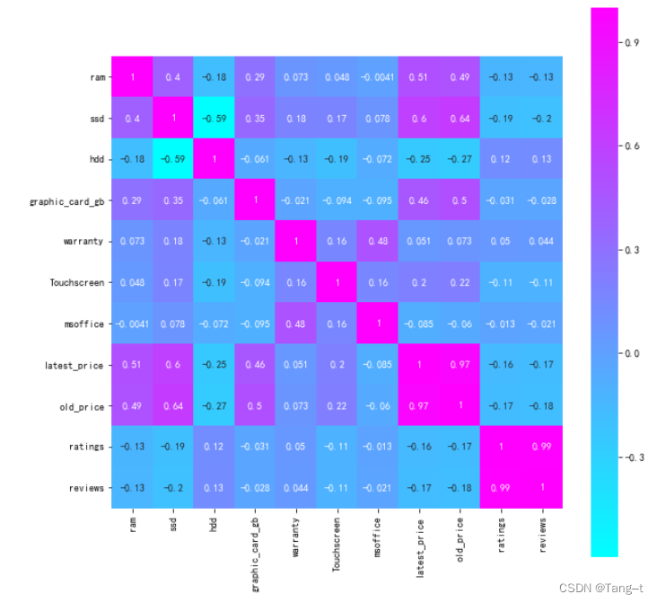

# 绘制最值得研究的5个变量的配对图
sns.pairplot(data[['latest_price', 'old_price', 'star_rating', 'ratings', 'reviews']],diag_kws={'color': 'navy'})
plt.show()

输出：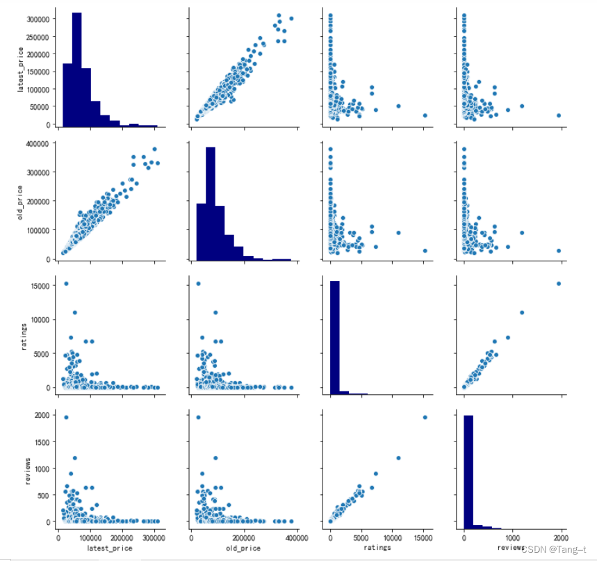

# 不同品牌电脑在售数量的柱状图
plt.figure(figsize=(12,6))
sns.countplot(x='brand', data=data)
plt.title('Number of Laptops for each Brand')
plt.show()

 输出：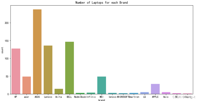

# 不同品牌电脑当前价格的箱型图
plt.figure(figsize=(12,6))
sns.boxplot(x='brand', y='latest_price', data=data)
plt.title('Latest Price of Laptops for each Brand')
plt.show()

 输出：

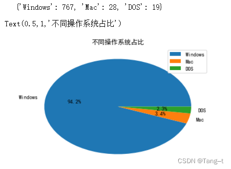
# 不同操作系统占比的饼图
shuliang = data['os'].value_counts().to_dict()
print(shuliang)
mc = list(shuliang.keys())
value = list(shuliang.values())
# 求百分率
value_bfl = [item / len(data) for item in value]
# 饼图绘制
plt.pie(value_bfl, labels=mc, autopct='%1.1f%%')
# 添加图例
plt.legend(mc, loc="best")
# 添加主题
plt.title("不同操作系统占比")

输出： 

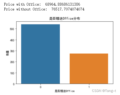
# 赠送Office的产品售价会不会高于不赠送的产品
office_present_price = data[data['msoffice'] == 1]['latest_price'].mean()
office_absent_price = data[data['msoffice'] == 0]['latest_price'].mean()

print("Price with Office: ", office_present_price)
print("Price without Office: ", office_absent_price)

# 是否赠送Office分布
sns.countplot(x='msoffice', data=data)
plt.xlabel('是否赠送Office')
plt.ylabel('数量')
plt.title('是否赠送Office分布')
plt.show()

输出： 

# 最受关注的10个笔记本产品
top_10_products = data.nlargest(10, 'reviews')
top_10_products

输出：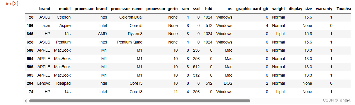

# 绘制电脑当前价格和上市价格的直方图和核密度图
plt.figure(figsize=(12,6))
sns.distplot(data['latest_price'], bins=20, kde=True)
plt.title('Histogram of Latest Price')
plt.show()

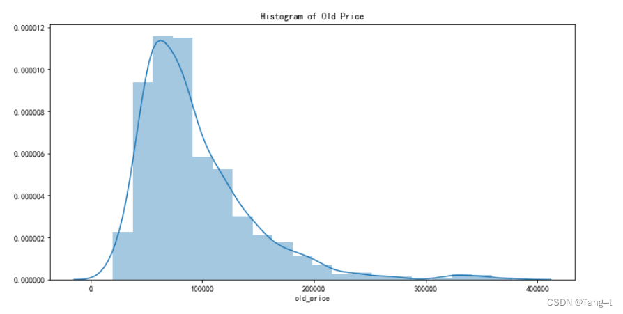
plt.figure(figsize=(12,6))
sns.distplot(data['old_price'].dropna(), bins=20, kde=True)
plt.title('Histogram of Old Price')
plt.show()

输出：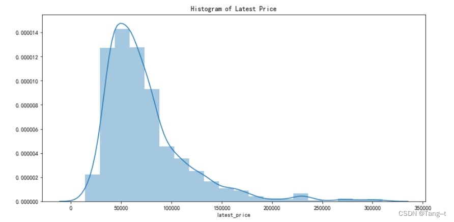

# from sklearn.linear_model import LinearRegression
from sklearn.model_selection import train_test_split

data1 = data1.dropna()

# 1. 删除无关列
X = data1.drop(columns=['brand', 'model', 'processor_name', 'latest_price', 'old_price'])

# 2. 对类别型特征进行编码
X = pd.get_dummies(X, columns=['processor_brand', 'os', 'weight'])

y1 = data1['latest_price']
y2 = data1['old_price'].dropna()

# 5. 用更新后的 X 和 y 重新创建训练集和测试集
X_train1, X_test1, y_train1, y_test1 = train_test_split(X, y1, test_size=0.2)
X_train2, X_test2, y_train2, y_test2 = train_test_split(X.loc[y2.index], y2, test_size=0.2)

reg1 = LinearRegression().fit(X_train1, y_train1)
reg2 = LinearRegression().fit(X_train2, y_train2)

# 查看系数和截距
print('Coefficients1: ', reg1.coef_)
print('Intercept1: ', reg1.intercept_)

# 查看系数和截距
print('Coefficients2: ', reg2.coef_)
print('Intercept2: ', reg2.intercept_)

print("Latest Price R^2: ", reg1.score(X_test1, y_test1))
print("Old Price R^2: ", reg2.score(X_test2, y_test2))

输出：

Coefficients1:  [-7.07557714e+03  3.35139679e+03  5.46847719e+01  1.13268707e+01
  1.44505278e+03  1.07945010e+04 -4.63938576e+03  2.59755273e+04
  4.86800940e+03  1.64308407e+01 -4.42821541e+00  8.29840136e+00
 -1.61474505e+03  1.61474505e+03  4.47998769e+04 -4.47998769e+04
 -8.18032776e+03  5.23072822e+03  2.94959954e+03]
Intercept1:  -39773.65850356128
Coefficients2:  [-2.86369354e+03  3.17034169e+03  5.61052151e+01  3.51677257e+00
  4.87360080e+03  8.18075518e+03 -3.10167810e+03  1.88745428e+04
  6.68445411e+03  1.09098471e+03  1.22262513e+00 -6.77852369e+01
  7.79344414e+02 -7.79344414e+02  4.14202603e+04 -4.14202603e+04
 -8.14263094e+03  3.51526774e+03  4.62736320e+03]
Intercept2:  -36357.18754110069
Latest Price R^2:  0.7161619386701985
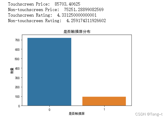
Old Price R^2:  0.7097949829352088

# 是否为触屏价格和评级的比较
data1['latest_price'] = data1['latest_price'].astype('float')
data1['star_rating'] = data1['star_rating'].astype('float')
touchscreen_price = data1[data1['Touchscreen'] == 1]['latest_price'].mean()
non_touchscreen_price = data1[data1['Touchscreen'] == 0]['latest_price'].mean()
touchscreen_rating = data1[data1['Touchscreen'] == 1]['star_rating'].mean()
non_touchscreen_rating = data1[data1['Touchscreen'] == 0]['star_rating'].mean()

print("Touchscreen Price: ", touchscreen_price)
print("Non-touchscreen Price: ", non_touchscreen_price)
print("Touchscreen Rating: ", touchscreen_rating)
print("Non-touchscreen Rating: ", non_touchscreen_rating)

# 是否触摸屏分布
sns.countplot(x='Touchscreen', data=data)
plt.xlabel('是否触摸屏')
plt.ylabel('数量')
plt.title('是否触摸屏分布')
plt.show()

输出： 

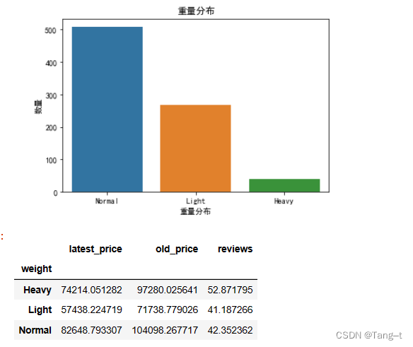
# 重量分析
data.groupby('weight')['latest_price','old_price','reviews'].mean()
# 重量分布
sns.countplot(x='weight', data=data)
plt.xlabel('重量分布')
plt.ylabel('数量')
plt.title('重量分布')
plt.show()
data.groupby('weight')['latest_price','old_price','reviews'].mean()

输出： 

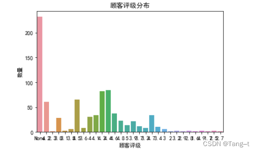
# 顾客评级分布
sns.countplot(x='star_rating', data=data)
plt.xlabel('顾客评级')
plt.ylabel('数量')
plt.title('顾客评级分布')
plt.show()

输出： 

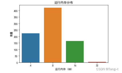
# 运行内存分布
sns.countplot(x='ram', data=data)
plt.xlabel('运行内存 (GB)')
plt.ylabel('数量')
plt.title('运行内存分布')
plt.show()

输出：