2024年最新关于面试的经典书籍推荐，人脸检测实战进阶：使用 OpenCV 进行活体检测，面试考场规则

收集整理了一份《2024年最新Python全套学习资料》免费送给大家，初衷也很简单，就是希望能够帮助到想自学提升又不知道该从何学起的朋友。

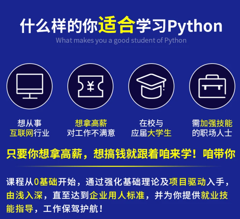
既有适合小白学习的零基础资料，也有适合3年以上经验的小伙伴深入学习提升的进阶课程，涵盖了95%以上Python知识点，真正体系化！

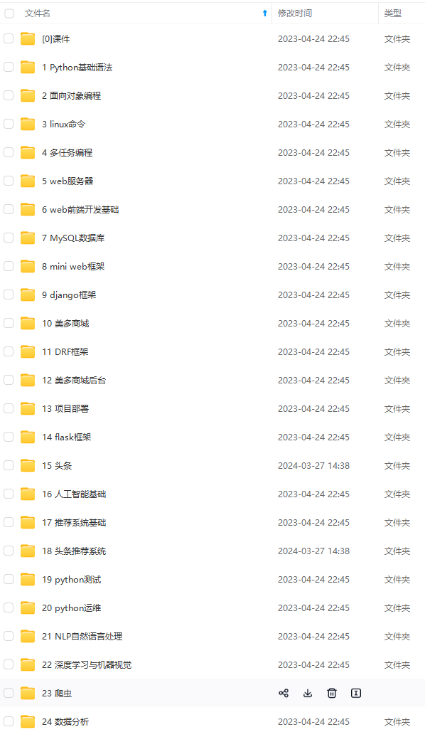
由于文件比较多，这里只是将部分目录截图出来

如果你需要这些资料，可以添加V无偿获取：hxbc188 （备注666）

正文

from tensorflow.keras.layers import MaxPooling2D

from tensorflow.keras.layers import Activation

from tensorflow.keras.layers import Flatten

from tensorflow.keras.layers import Dropout

from tensorflow.keras.layers import Dense

from tensorflow.keras import backend as K

class LivenessNet:

@staticmethod

def build(width, height, depth, classes):

initialize the model along with the input shape to be

“channels last” and the channels dimension itself

model = Sequential()

inputShape = (height, width, depth)

chanDim = -1

if we are using “channels first”, update the input shape

and channels dimension

if K.image_data_format() == “channels_first”:

inputShape = (depth, height, width)

chanDim = 1

导入包。 要深入了解这些层和功能中的每一个，请务必参考使用 Python 进行计算机视觉深度学习。

定义 LivenessNet 类。它包含一个静态方法 build。 build 方法接受四个参数：

• width ：图像/体积的宽度。

• height ：图像有多高。

• depth ：图像的通道数（在本例中为 3，因为我们将使用 RGB 图像）。

• classes：类别的数量。 我们总共有两个类：“real”和“fake”。

初始化模型。 定义inputShape ，而通道排序。 让我们开始向我们的 CNN 添加层：

first CONV => RELU => CONV => RELU => POOL layer set

model.add(Conv2D(16, (3, 3), padding=“same”,

input_shape=inputShape))

model.add(Activation(“relu”))

model.add(BatchNormalization(axis=chanDim))

model.add(Conv2D(16, (3, 3), padding=“same”))

model.add(Activation(“relu”))

model.add(BatchNormalization(axis=chanDim))

model.add(MaxPooling2D(pool_size=(2, 2)))

model.add(Dropout(0.25))

second CONV => RELU => CONV => RELU => POOL layer set

model.add(Conv2D(32, (3, 3), padding=“same”))

model.add(Activation(“relu”))

model.add(BatchNormalization(axis=chanDim))

model.add(Conv2D(32, (3, 3), padding=“same”))

model.add(Activation(“relu”))

model.add(BatchNormalization(axis=chanDim))

model.add(MaxPooling2D(pool_size=(2, 2)))

model.add(Dropout(0.25))

CNN网络类似VGG。 它非常浅，只有几个学习过的过滤器。 理想情况下，我们不需要深度网络来区分真实和欺骗的面孔。

第一个 CONV => RELU => CONV => RELU => POOL 层，其中还添加了批量归一化和 dropout。 第二个 CONV => RELU => CONV => RELU => POOL 层。 最后，我们将添加我们的 FC => RELU 层：

first (and only) set of FC => RELU layers

model.add(Flatten())

model.add(Dense(64))

model.add(Activation(“relu”))

model.add(BatchNormalization())

model.add(Dropout(0.5))

softmax classifier

model.add(Dense(classes))

model.add(Activation(“softmax”))

return the constructed network architecture

return model

全连接层和 ReLU 激活层组成，带有 softmax 分类器头。

模型返回。

创建活体检测器训练脚本

======================================================================

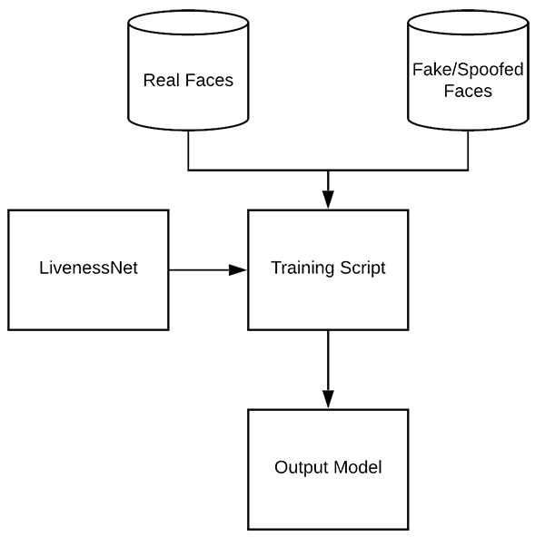
鉴于我们的真实/欺骗图像数据集以及 LivenessNet 的实现，我们现在准备训练网络。 打开 train.py 文件并插入以下代码：

set the matplotlib backend so figures can be saved in the background

import matplotlib

matplotlib.use(“Agg”)

import the necessary packages

from pyimagesearch.livenessnet import LivenessNet

from sklearn.preprocessing import LabelEncoder

from sklearn.model_selection import train_test_split

from sklearn.metrics import classification_report

from tensorflow.keras.preprocessing.image import ImageDataGenerator

from tensorflow.keras.optimizers import Adam

from tensorflow.keras.utils import to_categorical

from imutils import paths

import matplotlib.pyplot as plt

import numpy as np

import argparse

import pickle

import cv2

import os

construct the argument parser and parse the arguments

ap = argparse.ArgumentParser()

ap.add_argument(“-d”, “–dataset”, required=True,

help=“path to input dataset”)

ap.add_argument(“-m”, “–model”, type=str, required=True,

help=“path to trained model”)

ap.add_argument(“-l”, “–le”, type=str, required=True,

help=“path to label encoder”)

ap.add_argument(“-p”, “–plot”, type=str, default=“plot.png”,

help=“path to output loss/accuracy plot”)

args = vars(ap.parse_args())

我们的面部活力训练脚本由许多导入（第 2-19 行）组成。现在让我们回顾一下：

• matplotlib ：用于生成训练图。我们指定了“Agg”后端，以便我们可以轻松地将我们的绘图保存到第 3 行的磁盘中。

• LivenessNet ：我们在上一节中定义的 liveness CNN。

• train_test_split ：来自 scikit-learn 的一个函数，它构建了我们的数据分割以进行训练和测试。 分类报告：同样来自 scikit-learn，该工具将生成关于我们模型性能的简要统计报告。

• ImageDataGenerator ：用于执行数据增强，为我们提供批量随机变异的图像。

• Adam ：一个非常适合这个模型的优化器。 （替代方法包括 SGD、RMSprop 等）。 路径：从我的 imutils 包中，该模块将帮助我们收集磁盘上所有图像文件的路径。

• pyplot ：用于生成一个很好的训练图。

• numpy ：Python 的数值处理库。这也是 OpenCV 的要求。

• argparse ：用于处理命令行参数。

• pickle ：用于将我们的标签编码器序列化到磁盘。

• cv2 ：我们的 OpenCV 绑定。

• os ：这个模块可以做很多事情，但我们只是将它用作操作系统路径分隔符。

查看脚本的其余部分应该更简单。 此脚本接受四个命令行参数：

• –dataset ：输入数据集的路径。 在这篇文章的前面，我们使用 gather_examples.py 脚本创建了数据集。

• –model ：我们的脚本将生成一个输出模型文件——在这里你提供它的路径。

• –le ：还需要提供输出序列化标签编码器文件的路径。

• –plot ：训练脚本将生成一个绘图。 如果你想覆盖 “plot.png” 的默认值，你应该在命令行中指定这个值。

下一个代码块将执行一些初始化并构建我们的数据：

initialize the initial learning rate, batch size, and number of

epochs to train for

INIT_LR = 1e-4

BS = 8

EPOCHS = 50

grab the list of images in our dataset directory, then initialize

the list of data (i.e., images) and class images

print(“[INFO] loading images…”)

imagePaths = list(paths.list_images(args[“dataset”]))

data = []

labels = []

loop over all image paths

for imagePath in imagePaths:

extract the class label from the filename, load the image and

resize it to be a fixed 32x32 pixels, ignoring aspect ratio

label = imagePath.split(os.path.sep)[-2]

image = cv2.imread(imagePath)

image = cv2.resize(image, (32, 32))

update the data and labels lists, respectively

data.append(image)

labels.append(label)

convert the data into a NumPy array, then preprocess it by scaling

all pixel intensities to the range [0, 1]

data = np.array(data, dtype=“float”) / 255.0

设置训练参数，包括初始学习率、批量大小和EPOCHS。

从那里，我们的 imagePaths 被抓取。 我们还初始化了两个列表来保存我们的数据和类标签。 循环构建我们的数据和标签列表。 数据由我们加载并调整为 32×32 像素的图像组成。 每个图像都有一个对应的标签存储在标签列表中。

所有像素强度都缩放到 [0, 1] 范围内，同时将列表制成 NumPy 数组。 现在让我们对标签进行编码并对数据进行分区：

encode the labels (which are currently strings) as integers and then

one-hot encode them

le = LabelEncoder()

labels = le.fit_transform(labels)

labels = to_categorical(labels, 2)

partition the data into training and testing splits using 75% of

the data for training and the remaining 25% for testing

(trainX, testX, trainY, testY) = train_test_split(data, labels,

test_size=0.25, random_state=42)

单热编码标签。 我们利用 scikit-learn 来划分我们的数据——75% 用于训练，而 25% 保留用于测试。 接下来，我们将初始化我们的数据增强对象并编译+训练我们的面部活力模型：

construct the training image generator for data augmentation

aug = ImageDataGenerator(rotation_range=20, zoom_range=0.15,

width_shift_range=0.2, height_shift_range=0.2, shear_range=0.15,

horizontal_flip=True, fill_mode=“nearest”)

initialize the optimizer and model

print(“[INFO] compiling model…”)

opt = Adam(lr=INIT_LR, decay=INIT_LR / EPOCHS)

model = LivenessNet.build(width=32, height=32, depth=3,

classes=len(le.classes_))

model.compile(loss=“binary_crossentropy”, optimizer=opt,

metrics=[“accuracy”])

train the network

print(“[INFO] training network for {} epochs…”.format(EPOCHS))

H = model.fit(x=aug.flow(trainX, trainY, batch_size=BS),

validation_data=(testX, testY), steps_per_epoch=len(trainX) // BS,

epochs=EPOCHS)

构造数据增强对象，该对象将生成具有随机旋转、缩放、移位、剪切和翻转的图像。

构建和编译LivenessNet 模型。 然后我们开始训练。 考虑到我们的浅层网络和小数据集，这个过程会相对较快。 一旦模型经过训练，我们就可以评估结果并生成训练图：

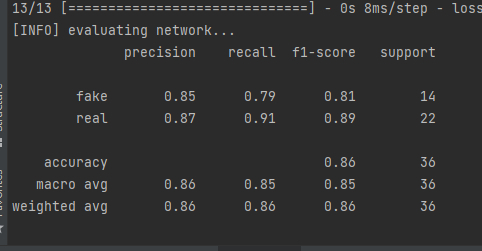
evaluate the network

print(“[INFO] evaluating network…”)

predictions = model.predict(x=testX, batch_size=BS)

print(classification_report(testY.argmax(axis=1),

predictions.argmax(axis=1), target_names=le.classes_))

save the network to disk

print(“[INFO] serializing network to ‘{}’…”.format(args[“model”]))

model.save(args[“model”], save_format=“h5”)

save the label encoder to disk

f = open(args[“le”], “wb”)

f.write(pickle.dumps(le))

f.close()

plot the training loss and accuracy

plt.style.use(“ggplot”)

plt.figure()

plt.plot(np.arange(0, EPOCHS), H.history[“loss”], label=“train_loss”)

plt.plot(np.arange(0, EPOCHS), H.history[“val_loss”], label=“val_loss”)

plt.plot(np.arange(0, EPOCHS), H.history[“accuracy”], label=“train_acc”)

plt.plot(np.arange(0, EPOCHS), H.history[“val_accuracy”], label=“val_acc”)

plt.title(“Training Loss and Accuracy on Dataset”)

plt.xlabel(“Epoch #”)

plt.ylabel(“Loss/Accuracy”)

plt.legend(loc=“lower left”)

plt.savefig(args[“plot”])

在测试集上进行预测。 从那里生成一个分类报告并将其打印到终端。 LivenessNet 模型与标签编码器一起序列化到磁盘。

生成训练历史图以供以后检查。

训练LivenessNet

========================================================================

python train.py --dataset dataset --model liveness.model --le le.pickle

使用 OpenCV 进行活体检测

===========================================================================

最后一步是组合所有部分：

• 我们将访问我们的网络摄像头/视频流

• 对每一帧应用人脸检测

• 对于检测到的每个人脸，应用我们的活体检测器模型

打开 liveness_demo.py 并插入以下代码：

import the necessary packages

from imutils.video import VideoStream

from tensorflow.keras.preprocessing.image import img_to_array

from tensorflow.keras.models import load_model

import numpy as np

import argparse

import imutils

import pickle

import time

import cv2

import os

construct the argument parser and parse the arguments

ap = argparse.ArgumentParser()

ap.add_argument(“-m”, “–model”, type=str, required=True,

help=“path to trained model”)

ap.add_argument(“-l”, “–le”, type=str, required=True,

help=“path to label encoder”)

ap.add_argument(“-d”, “–detector”, type=str, required=True,

help=“path to OpenCV’s deep learning face detector”)

ap.add_argument(“-c”, “–confidence”, type=float, default=0.5,

help=“minimum probability to filter weak detections”)

args = vars(ap.parse_args())

导入我们需要的包。 值得注意的是，我们将使用 -

• VideoStream 以访问我们的相机提要。

• img_to_array 以便我们的框架采用兼容的数组格式。

• load_model 加载我们序列化的 Keras 模型。

• imutils 的便利功能。

• cv2 用于我们的 OpenCV 绑定。

让我们解析我们的命令行参数：

• –model ：我们用于活体检测的预训练 Keras 模型的路径。

• –le ：我们到标签编码器的路径。

• –detector ：OpenCV 的深度学习人脸检测器的路径，用于查找人脸 ROI。

• –confidence ：过滤掉弱检测的最小概率阈值。

现在让我们继续初始化人脸检测器、LivenessNet 模型 + 标签编码器和我们的视频流：

load our serialized face detector from disk

print(“[INFO] loading face detector…”)

protoPath = os.path.sep.join([args[“detector”], “deploy.prototxt”])

modelPath = os.path.sep.join([args[“detector”],

“res10_300x300_ssd_iter_140000.caffemodel”])

net = cv2.dnn.readNetFromCaffe(protoPath, modelPath)

load the liveness detector model and label encoder from disk

print(“[INFO] loading liveness detector…”)

model = load_model(args[“model”])

le = pickle.loads(open(args[“le”], “rb”).read())

initialize the video stream and allow the camera sensor to warmup

print(“[INFO] starting video stream…”)

vs = VideoStream(src=0).start()

time.sleep(2.0)

OpenCV 加载人脸检测器通。

从那里我们加载我们的序列化、预训练模型 (LivenessNet) 和标签编码器。 我们的 VideoStream 对象被实例化，我们的相机被允许预热两秒钟。 在这一点上，是时候开始遍历帧来检测真人脸与假人脸/欺骗人脸了：

loop over the frames from the video stream

while True:

grab the frame from the threaded video stream and resize it

to have a maximum width of 600 pixels

frame = vs.read()

frame = imutils.resize(frame, width=600)

grab the frame dimensions and convert it to a blob

(h, w) = frame.shape[:2]

blob = cv2.dnn.blobFromImage(cv2.resize(frame, (300, 300)), 1.0,

(300, 300), (104.0, 177.0, 123.0))

pass the blob through the network and obtain the detections and

predictions

net.setInput(blob)

detections = net.forward()

打开一个无限 while 循环块，我们从捕获和调整单个帧的大小开始。

调整大小后，会抓取框架的尺寸，以便我们稍后执行缩放。 使用 OpenCV 的 blobFromImage 函数，我们生成一个 blob，然后通过将其传递到人脸检测器网络来继续执行推理。

现在我们准备好迎接有趣的部分——使用 OpenCV 和深度学习进行活体检测：

loop over the detections

for i in range(0, detections.shape[2]):

extract the confidence (i.e., probability) associated with the

prediction

confidence = detections[0, 0, i, 2]

filter out weak detections

if confidence > args[“confidence”]:

compute the (x, y)-coordinates of the bounding box for

the face and extract the face ROI

box = detections[0, 0, i, 3:7] * np.array([w, h, w, h])

(startX, startY, endX, endY) = box.astype(“int”)

ensure the detected bounding box does fall outside the

dimensions of the frame

startX = max(0, startX)

startY = max(0, startY)

endX = min(w, endX)

endY = min(h, endY)

extract the face ROI and then preproces it in the exact

same manner as our training data

face = frame[startY:endY, startX:endX]

face = cv2.resize(face, (32, 32))

face = face.astype(“float”) / 255.0

face = img_to_array(face)

face = np.expand_dims(face, axis=0)

pass the face ROI through the trained liveness detector

model to determine if the face is “real” or “fake”

preds = model.predict(face)[0]

j = np.argmax(preds)

label = le.classes_[j]

draw the label and bounding box on the frame

label = “{}: {:.4f}”.format(label, preds[j])

cv2.putText(frame, label, (startX, startY - 10),

cv2.FONT_HERSHEY_SIMPLEX, 0.5, (0, 0, 255), 2)

cv2.rectangle(frame, (startX, startY), (endX, endY),

(0, 0, 255), 2)

遍历人脸检测。 在循环里面：

• 过滤掉弱检测。

• 提取人脸边界框坐标并确保它们不超出框架的尺寸。

• 提取人脸 ROI 并以与我们的训练数据相同的方式对其进行预处理。

• 使用我们的活体检测器模型来确定面部是“真实的”还是“假的/欺骗的”。

• 接下来是您插入自己的代码以执行人脸识别的地方，但仅限于真实图像。 伪代码类似于 if label == “real”: run_face_reconition() ）。

• 最后（对于这个演示），我们在脸部周围绘制标签文本和一个矩形。

让我们显示我们的结果并清理：

show the output frame and wait for a key press

cv2.imshow(“Frame”, frame)

key = cv2.waitKey(1) & 0xFF

if the q key was pressed, break from the loop

if key == ord(“q”):

break

do a bit of cleanup

cv2.destroyAllWindows()

vs.stop()

将我们的活体检测器部署到实时视频中

============================================================================

打开一个终端并执行以下命令：

python liveness_demo.py --model liveness.model --le le.pickle \

一、Python所有方向的学习路线

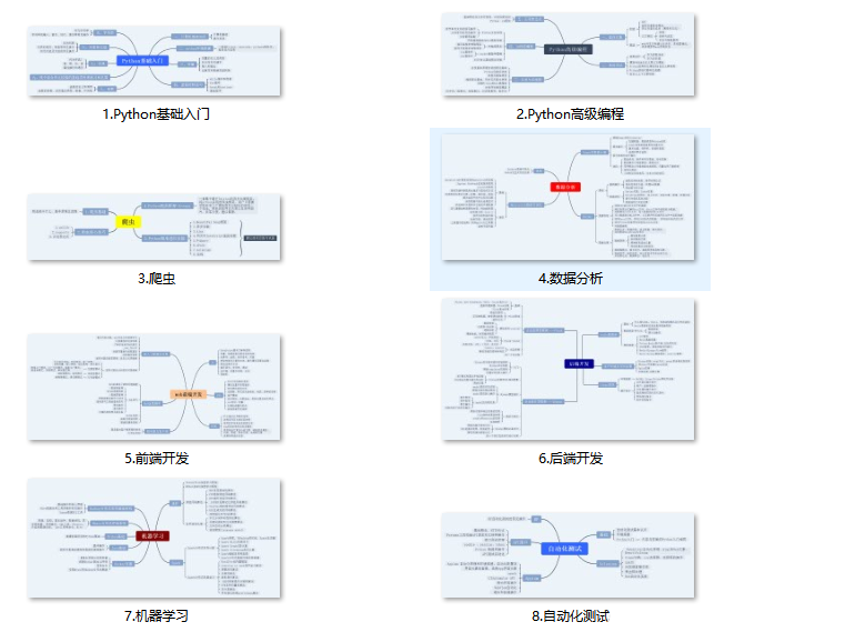
Python所有方向的技术点做的整理，形成各个领域的知识点汇总，它的用处就在于，你可以按照下面的知识点去找对应的学习资源，保证自己学得较为全面。

二、Python必备开发工具

工具都帮大家整理好了，安装就可直接上手！

三、最新Python学习笔记

当我学到一定基础，有自己的理解能力的时候，会去阅读一些前辈整理的书籍或者手写的笔记资料，这些笔记详细记载了他们对一些技术点的理解，这些理解是比较独到，可以学到不一样的思路。

四、Python视频合集

观看全面零基础学习视频，看视频学习是最快捷也是最有效果的方式，跟着视频中老师的思路，从基础到深入，还是很容易入门的。

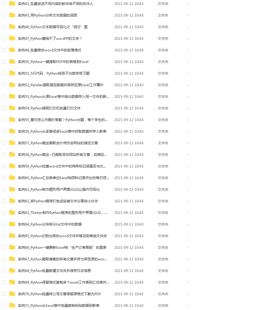
五、实战案例

纸上得来终觉浅，要学会跟着视频一起敲，要动手实操，才能将自己的所学运用到实际当中去，这时候可以搞点实战案例来学习。

六、面试宝典

简历模板

网上学习资料一大堆，但如果学到的知识不成体系，遇到问题时只是浅尝辄止，不再深入研究，那么很难做到真正的技术提升。

如果你需要这些资料，可以添加V无偿获取：hxbc188 （备注666）

一个人可以走的很快，但一群人才能走的更远！不论你是正从事IT行业的老鸟或是对IT行业感兴趣的新人，都欢迎加入我们的的圈子（技术交流、学习资源、职场吐槽、大厂内推、面试辅导），让我们一起学习成长！
(https://img-blog.csdnimg.cn/6d414e9f494742db8bcc3fa312200539.png)

四、Python视频合集

观看全面零基础学习视频，看视频学习是最快捷也是最有效果的方式，跟着视频中老师的思路，从基础到深入，还是很容易入门的。

五、实战案例

纸上得来终觉浅，要学会跟着视频一起敲，要动手实操，才能将自己的所学运用到实际当中去，这时候可以搞点实战案例来学习。

六、面试宝典

简历模板

网上学习资料一大堆，但如果学到的知识不成体系，遇到问题时只是浅尝辄止，不再深入研究，那么很难做到真正的技术提升。

如果你需要这些资料，可以添加V无偿获取：hxbc188 （备注666）
[外链图片转存中…(img-ruUZx8pK-1713858059906)]

一个人可以走的很快，但一群人才能走的更远！不论你是正从事IT行业的老鸟或是对IT行业感兴趣的新人，都欢迎加入我们的的圈子（技术交流、学习资源、职场吐槽、大厂内推、面试辅导），让我们一起学习成长！