【图像融合】基于剪切变换和平均亮度的图像融合算法研究附matlab代码

 ✅作者简介：热爱科研的Matlab仿真开发者，擅长数据处理、建模仿真、程序设计、完整代码获取、论文复现及科研仿真。

🍎 往期回顾关注个人主页：Matlab科研工作室

🍊个人信条：格物致知,完整Matlab代码及仿真咨询内容私信。

🔥 内容介绍

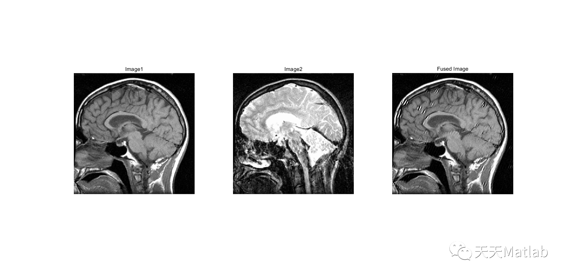
图像融合是计算机视觉领域的一个重要研究方向，旨在将多幅图像融合成一幅更具信息丰富度和视觉效果的图像。本文将介绍一种基于剪切变换和平均亮度的图像融合算法，并详细阐述其算法步骤。

图像融合算法的目标是将多幅图像中的有用信息进行合理的融合，以产生一幅更好的图像。该算法的步骤主要包括：图像预处理、剪切变换、亮度调整和图像合成。

首先，进行图像预处理。这一步骤主要是对待融合的图像进行一些基本的处理，如调整图像大小、去除噪声等。预处理的目的是为了提高后续步骤的处理效果。

接下来是剪切变换。该步骤的目的是将待融合的图像进行剪切，以使它们的边缘对齐。剪切变换可以通过寻找两幅图像之间的共同特征点，并进行相应的变换来实现。这样做的好处是能够减少融合后图像的失真程度，提高融合效果。

然后是亮度调整。在剪切变换之后，由于图像的亮度可能存在差异，需要对图像的亮度进行调整，以使它们的亮度更加一致。常用的亮度调整方法包括直方图均衡化和灰度拉伸等。通过亮度调整，可以使融合后的图像更加自然和逼真。

最后是图像合成。在经过前面的步骤之后，可以将剪切变换和亮度调整后的图像进行融合。常用的图像融合方法有加权平均法和多分辨率融合法等。加权平均法是将待融合的图像按照一定的权重进行加权平均，得到最终的融合图像。多分辨率融合法是将图像分解成不同的分辨率层次，然后对每个层次进行融合，最后再进行重建。这些方法可以根据实际需求选择，以获得最佳的融合效果。

综上所述，基于剪切变换和平均亮度的图像融合算法是一种有效的图像融合方法。通过对图像进行剪切变换和亮度调整，以及采用合适的图像合成方法，可以得到一幅更具信息丰富度和视觉效果的融合图像。这种算法在计算机视觉领域有着广泛的应用前景，可以用于图像增强、目标检测等方面，具有重要的研究和实际价值。

📣 部分代码

addpath(genpath('ShearLab3D'))​% 读取图像img1 = imread('c07_1.tif');img2 = imread('c07_2.tif');​% 调整图像尺寸figure(1);img1 = imresize(img1,[512,512]);imshow(img1);title('Image1');figure(2);img2 = imresize(img2,[512,512]);imshow(img2);title('Image2');oeffs_fused,shearletSystem);​% 显示融合图像figure(3);imshow(uint8(fused_image));title('Fused Image');​% 原图像original1 = double(img1);original2 = double(img2);​% Peak Signal-to-Noise Ratio (PSNR)% psnr1 = psnr(fused_image, original1);% psnr2 = psnr(fused_image, original2);psnr1 = calculate_psnr(fused_image, original1);psnr2 = calculate_psnr(fused_image, original2);fprintf('PSNR for image 1: %f\n', psnr1);fprintf('PSNR for image 2: %f\n', psnr2);​% Structural Similarity Index (SSIM)ssim1 = ssim(fused_image, original1);ssim2 = ssim(fused_image, original2);fprintf('SSIM for image 1: %f\n', ssim1);fprintf('SSIM for image 2: %f\n', ssim2);​% % Mean Squared Error (MSE)% mse1 = immse(fused_image, original1);% mse2 = immse(fused_image, original2);% fprintf('MSE for image 1: %f\n', mse1);% fprintf('MSE for image 2: %f\n', mse2);% % % Mean Absolute Difference (MAD)% mad1 = mean(abs(fused_image(:) - original1(:)));% mad2 = mean(abs(fused_image(:) - original2(:)));% fprintf('MAD for image 1: %f\n', mad1);% fprintf('MAD for image 2: %f\n', mad2);% % % NCC% ncc_value1 = NCC(fused_image, original1);% ncc_value2 = NCC(fused_image, original2);% fprintf('NCC for image 1: %f\n', ncc_value1);% fprintf('NCC for image 2: %f\n', ncc_value2);% % % MAE% mae_value1 = MAE(fused_image, original1);% mae_value2 = MAE(fused_image, original2);% fprintf('MAE for image 1: %f\n', mae_value1);% fprintf('MAE for image 2: %f\n', mae_value2);​% Compute the standard deviationsd_fused = std(double(fused_image(:)));fprintf('SD of fused image: %f\n', sd_fused);​% Spatial Frequencysf = mean(abs(diff(double(fused_image), 1, 1)), 'all') + mean(abs(diff(double(fused_image), 1, 2)), 'all');fprintf('Spatial Frequency of fused image: %f\n', sf);​% Average Gradient[gradX, gradY] = gradient(double(fused_image));ag = mean(sqrt(gradX.^2 + gradY.^2), 'all');fprintf('Average Gradient of fused image: %f\n', ag);​% Information Entropyie = entropy(fused_image);fprintf('Information Entropy of fused image: %f\n', ie);​% Mutual Informationmi1 = mi(double(original1), double(fused_image));fprintf('Mutual Information of fused image and original image 1: %f\n', mi1);mi2 = mi(double(original2), double(fused_image));fprintf('Mutual Information of fused image and original image 2: %f\n', mi2);​​​% Additional functionsfunction ncc = NCC(img1, img2)    img1 = img1 - mean(img1(:));    img2 = img2 - mean(img2(:));    numerator = sum(sum(img1 .* img2));    denominator = sqrt(sum(sum(img1 .^ 2)) * sum(sum(img2 .^ 2)));    ncc = numerator / denominator;end​function mae = MAE(target, reference)    error = target - reference;    mae = mean(abs(error(:)));end​% Define the Mutual Information functionfunction h = mi(A,B)  A = round((A - min(A(:))) / (max(A(:)) - min(A(:))) * 255);  B = round((B - min(B(:))) / (max(B(:)) - min(B(:))) * 255);  jointHistogram = accumarray([A(:) B(:)]+1, 1) / numel(A);  jointEntropy = - sum(jointHistogram(jointHistogram > 0) .* log2(jointHistogram(jointHistogram > 0)));  entropyA = entropy(uint8(A));  entropyB = entropy(uint8(B));  h = entropyA + entropyB - jointEntropy;end​function psnr_val = calculate_psnr(img1, img2)    img1 = double(img1);    img2 = double(img2);    mse = mean((img1(:) - img2(:)).^2);    if mse == 0        psnr_val = Inf;    else        maxValue = double(max(img1(:)));        psnr_val = 20 * log10(maxValue/sqrt(mse));    endend​

⛳️ 运行结果

🔗 参考文献

[1] 徐领章.基于TMS320DM6467的红外与微光图像融合算法研究[D].云南师范大学,2016.

[2] 杨金库.基于二维经验模态分解的图像融合算法研究[D].西北工业大学[2023-10-27].DOI:CNKI:CDMD:1.1017.803623.

[3] 吴璐璐.基于小波变换域的视频水印算法研究[D].江西理工大学,2013.

🎈 部分理论引用网络文献，若有侵权联系博主删除

🎁  关注我领取海量matlab电子书和数学建模资料

👇  私信完整代码、论文复现、期刊合作、论文辅导及科研仿真定制

1 各类智能优化算法改进及应用

生产调度、经济调度、装配线调度、充电优化、车间调度、发车优化、水库调度、三维装箱、物流选址、货位优化、公交排班优化、充电桩布局优化、车间布局优化、集装箱船配载优化、水泵组合优化、解医疗资源分配优化、设施布局优化、可视域基站和无人机选址优化

2 机器学习和深度学习方面

卷积神经网络（CNN）、LSTM、支持向量机（SVM）、最小二乘支持向量机（LSSVM）、极限学习机（ELM）、核极限学习机（KELM）、BP、RBF、宽度学习、DBN、RF、RBF、DELM、XGBOOST、TCN实现风电预测、光伏预测、电池寿命预测、辐射源识别、交通流预测、负荷预测、股价预测、PM2.5浓度预测、电池健康状态预测、水体光学参数反演、NLOS信号识别、地铁停车精准预测、变压器故障诊断

2.图像处理方面

图像识别、图像分割、图像检测、图像隐藏、图像配准、图像拼接、图像融合、图像增强、图像压缩感知

3 路径规划方面

旅行商问题（TSP）、车辆路径问题（VRP、MVRP、CVRP、VRPTW等）、无人机三维路径规划、无人机协同、无人机编队、机器人路径规划、栅格地图路径规划、多式联运运输问题、车辆协同无人机路径规划、天线线性阵列分布优化、车间布局优化

4 无人机应用方面

无人机路径规划、无人机控制、无人机编队、无人机协同、无人机任务分配、无人机安全通信轨迹在线优化

5 无线传感器定位及布局方面

传感器部署优化、通信协议优化、路由优化、目标定位优化、Dv-Hop定位优化、Leach协议优化、WSN覆盖优化、组播优化、RSSI定位优化

6 信号处理方面

信号识别、信号加密、信号去噪、信号增强、雷达信号处理、信号水印嵌入提取、肌电信号、脑电信号、信号配时优化

7 电力系统方面

微电网优化、无功优化、配电网重构、储能配置

8 元胞自动机方面

交通流 人群疏散 病毒扩散 晶体生长

9 雷达方面

卡尔曼滤波跟踪、航迹关联、航迹融合