


目录
作业1
编程实现
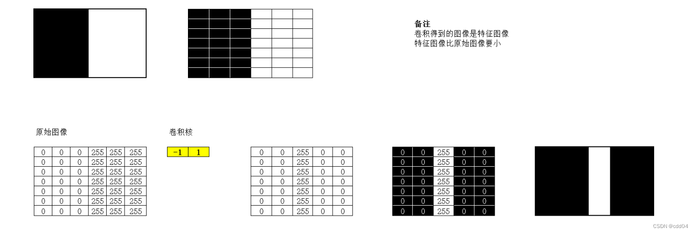

1. 图1使用卷积核,输出特征图
import torch
import torch.nn.functional as F
import matplotlib.pyplot as plt

featuremap=torch.tensor([[0,0,0,255,255,255],
                      [0,0,0,255,255,255],
                      [0,0,0,255,255,255],
                      [0,0,0,255,255,255],
                      [0,0,0,255,255,255]])
#确定卷积网络
class Cnet(torch.nn.Module):
    def __init__(self,filter,kshape):
        super(Cnet, self).__init__()
        filter = torch.reshape(filter,kshape)
        self.weight = torch.nn.Parameter(data=filter, requires_grad=False)
    def forward(self, featuremap):
        featuremap = F.conv2d(featuremap,self.weight,stride=1,padding=0)
        return  featuremap
#确定卷积层
filter=torch.tensor([-1,1])
#更改卷积层的形状适应卷积函数
kshape = (1,1,1,2)
#生成模型
model = Cnet(filter=filter,kshape=kshape)
#更改图片的形状适应卷积层
featuremap = torch.reshape(featuremap,(1,1,5,6))
output = model(featuremap)
output = torch.reshape(output,(5,5))
plt.imshow(output,cmap='gray')
plt.show()
2. 图1使用卷积核
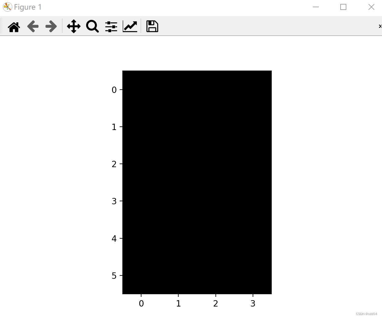
,输出特征图
import torch
import torch.nn.functional as F
import matplotlib.pyplot as plt

featuremap=torch.tensor([[0,0,0,255,255,255],
                      [0,0,0,255,255,255],
                      [0,0,0,255,255,255],
                      [0,0,0,255,255,255],
                      [0,0,0,255,255,255]])
#确定卷积网络
class Cnet(torch.nn.Module):
    def __init__(self,filter,kshape):
        super(Cnet, self).__init__()
        filter = torch.reshape(filter,kshape)
        self.weight = torch.nn.Parameter(data=filter, requires_grad=False)
    def forward(self, featuremap):
        featuremap = F.conv2d(featuremap,self.weight,stride=1,padding=0)
        return  featuremap
#确定卷积层
filter=torch.tensor([-1,1])
#更改卷积层的形状适应卷积函数
kshape = (1,1,2,1)
#生成模型
model = Cnet(filter=filter,kshape=kshape)
#更改图片的形状适应卷积层
featuremap = torch.reshape(featuremap,(1,1,5,6))
output = model(featuremap)
output = torch.reshape(output,(6,4))
plt.imshow(output,cmap='gray')
plt.show()
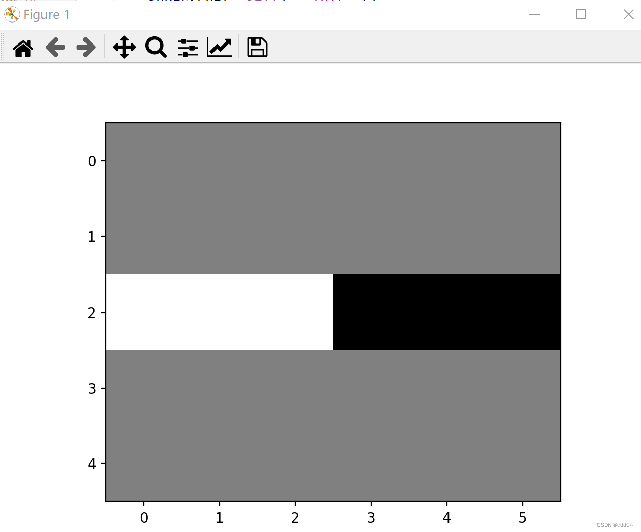
3. 图2使用卷积核,输出特征图
import torch
import torch.nn.functional as F
import matplotlib.pyplot as plt

featuremap=torch.tensor([[0,0,0,255,255,255],
                      [0,0,0,255,255,255],
                      [0,0,0,255,255,255],
                      [255,255,255,0,0,0],
                      [255,255,255,0,0,0],
                      [255,255,255,0,0,0]])
#确定卷积网络
class Cnet(torch.nn.Module):
    def __init__(self,filter,kshape):
        super(Cnet, self).__init__()
        filter = torch.reshape(filter,kshape)
        self.weight = torch.nn.Parameter(data=filter, requires_grad=False)
    def forward(self, featuremap):
        featuremap = F.conv2d(featuremap,self.weight,stride=1,padding=0)
        return  featuremap
#确定卷积层
filter=torch.tensor([-1,1])
#更改卷积层的形状适应卷积函数
kshape = (1,1,1,2)
#生成模型
model = Cnet(filter=filter,kshape=kshape)
#更改图片的形状适应卷积层
featuremap = torch.reshape(featuremap,(1,1,6,6))
output = model(featuremap)
output = torch.reshape(output,(6,5))
plt.imshow(output,cmap='gray')
plt.show()
 4. 图2使用卷积核
,输出特征图
import torch
import torch.nn.functional as F
import matplotlib.pyplot as plt

featuremap=torch.tensor([[0,0,0,255,255,255],
                      [0,0,0,255,255,255],
                      [0,0,0,255,255,255],
                      [255,255,255,0,0,0],
                      [255,255,255,0,0,0],
                      [255,255,255,0,0,0]])
#确定卷积网络
class Cnet(torch.nn.Module):
    def __init__(self,filter,kshape):
        super(Cnet, self).__init__()
        filter = torch.reshape(filter,kshape)
        self.weight = torch.nn.Parameter(data=filter, requires_grad=False)
    def forward(self, featuremap):
        featuremap = F.conv2d(featuremap,self.weight,stride=1,padding=0)
        return  featuremap
#确定卷积层
filter=torch.tensor([-1,1])
#更改卷积层的形状适应卷积函数
kshape = (1,1,2,1)
#生成模型
model = Cnet(filter=filter,kshape=kshape)
#更改图片的形状适应卷积层
featuremap = torch.reshape(featuremap,(1,1,6,6))
output = model(featuremap)
output = torch.reshape(output,(5,6))
plt.imshow(output,cmap='gray')
plt.show()
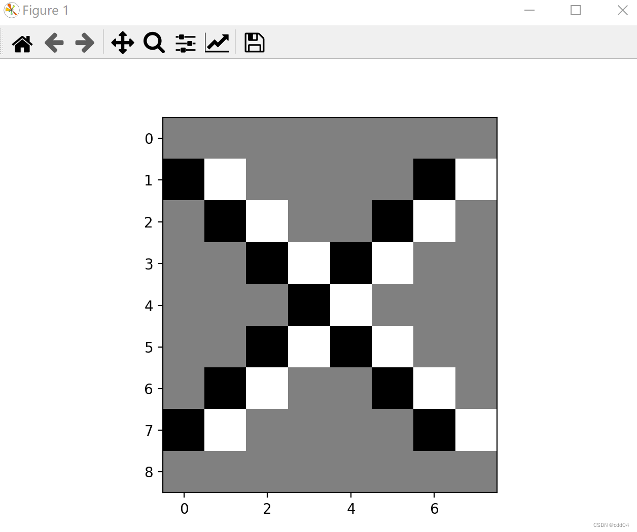
5. 图3使用卷积核,
,
,输出特征图
import torch
import torch.nn.functional as F
import matplotlib.pyplot as plt

featuremap=torch.tensor([[255,255,255,255,255,255,255,255,255],
                      [255,0  ,255,255,255,255,255,0  ,255],
                      [255,255,0  ,255,255,255,0  ,255,255],
                      [255,255,255,0  ,255,0  ,255,255,255],
                      [255,255,255,255,0  ,255,255,255,255],
                      [255,255,255,0  ,255,0  ,255,255,255],
                      [255,255,0  ,255,255,255,0  ,255,255],
                      [255,0  ,255,255,255,255,255,0  ,255],
                      [255,255,255,255,255,255,255,255,255],])
#确定卷积网络
class Cnet(torch.nn.Module):
    def __init__(self,filter,kshape):
        super(Cnet, self).__init__()
        filter = torch.reshape(filter,kshape)
        self.weight = torch.nn.Parameter(data=filter, requires_grad=False)
    def forward(self, featuremap):
        featuremap = F.conv2d(featuremap,self.weight,stride=1,padding=0)
        return  featuremap
#确定卷积层
filter=torch.tensor([-1,1])
#更改卷积层的形状适应卷积函数
kshape = (1,1,1,2)
#生成模型
model = Cnet(filter=filter,kshape=kshape)
#更改图片的形状适应卷积层
featuremap = torch.reshape(featuremap,(1,1,9,9))
output = model(featuremap)
output = torch.reshape(output,(9,8))
plt.imshow(output,cmap='gray')
plt.show()
import torch
import torch.nn.functional as F
import matplotlib.pyplot as plt

featuremap=torch.tensor([[255,255,255,255,255,255,255,255,255],
                      [255,0  ,255,255,255,255,255,0  ,255],
                      [255,255,0  ,255,255,255,0  ,255,255],
                      [255,255,255,0  ,255,0  ,255,255,255],
                      [255,255,255,255,0  ,255,255,255,255],
                      [255,255,255,0  ,255,0  ,255,255,255],
                      [255,255,0  ,255,255,255,0  ,255,255],
                      [255,0  ,255,255,255,255,255,0  ,255],
                      [255,255,255,255,255,255,255,255,255],])
#确定卷积网络
class Cnet(torch.nn.Module):
    def __init__(self,filter,kshape):
        super(Cnet, self).__init__()
        filter = torch.reshape(filter,kshape)
        self.weight = torch.nn.Parameter(data=filter, requires_grad=False)
    def forward(self, featuremap):
        featuremap = F.conv2d(featuremap,self.weight,stride=1,padding=0)
        return  featuremap
#确定卷积层
filter=torch.tensor([-1,1])
#更改卷积层的形状适应卷积函数
kshape = (1,1,2,1)
#生成模型
model = Cnet(filter=filter,kshape=kshape)
#更改图片的形状适应卷积层
featuremap = torch.reshape(featuremap,(1,1,9,9))
output = model(featuremap)
output = torch.reshape(output,(8,9))
plt.imshow(output,cmap='gray')
plt.show()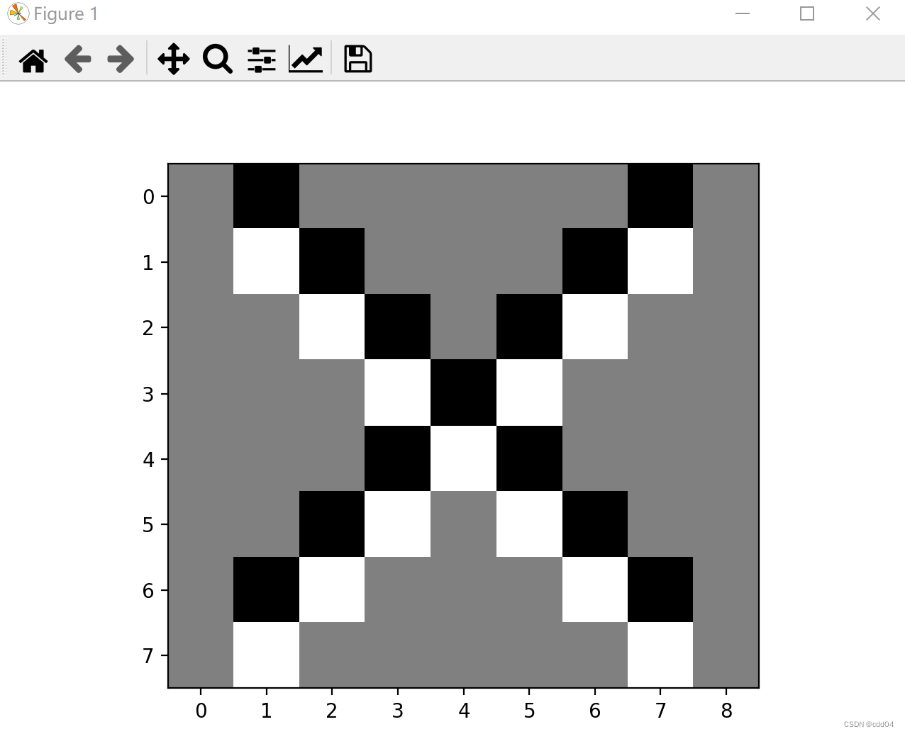
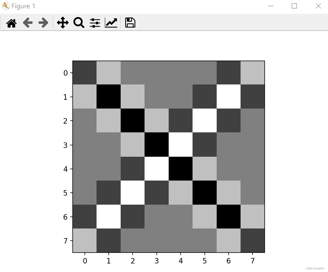
import torch
import torch.nn.functional as F
import matplotlib.pyplot as plt

featuremap=torch.tensor([[255,255,255,255,255,255,255,255,255],
                      [255,0  ,255,255,255,255,255,0  ,255],
                      [255,255,0  ,255,255,255,0  ,255,255],
                      [255,255,255,0  ,255,0  ,255,255,255],
                      [255,255,255,255,0  ,255,255,255,255],
                      [255,255,255,0  ,255,0  ,255,255,255],
                      [255,255,0  ,255,255,255,0  ,255,255],
                      [255,0  ,255,255,255,255,255,0  ,255],
                      [255,255,255,255,255,255,255,255,255],])
#确定卷积网络
class Cnet(torch.nn.Module):
    def __init__(self,filter,kshape):
        super(Cnet, self).__init__()
        filter = torch.reshape(filter,kshape)
        self.weight = torch.nn.Parameter(data=filter, requires_grad=False)
    def forward(self, featuremap):
        featuremap = F.conv2d(featuremap,self.weight,stride=1,padding=0)
        return  featuremap
#确定卷积层
filter=torch.tensor([[1,-1],
                       [-1,1]])
#更改卷积层的形状适应卷积函数
kshape = (1,1,2,2)
#生成模型
model = Cnet(filter=filter,kshape=kshape)
#更改图片的形状适应卷积层
featuremap = torch.reshape(featuremap,(1,1,9,9))
output = model(featuremap)
output = torch.reshape(output,(8,8))
plt.imshow(output,cmap='gray')
plt.show()
作业2
一、概念
用自己的语言描述“卷积、卷积核、特征图、特征选择、步长、填充、感受野”。
卷积:
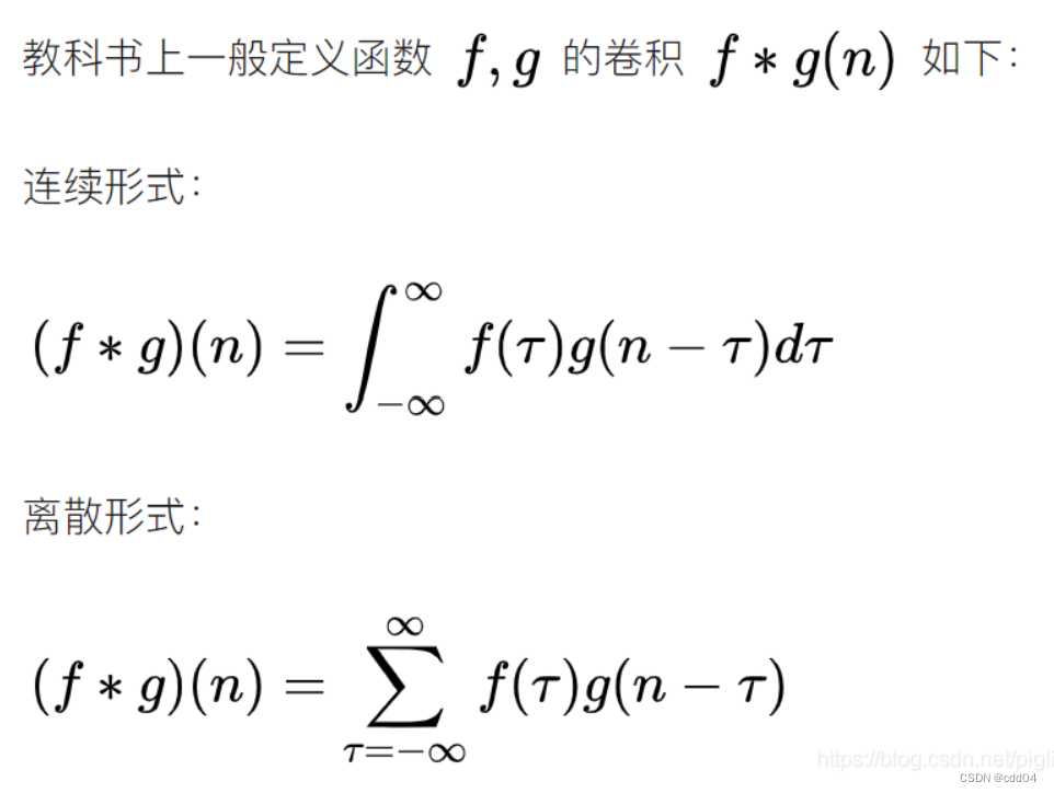
所谓两个函数的卷积,本质上就是先将一个函数翻转,然后进行滑动叠加。
在连续情况下,叠加指的是对两个函数的乘积求积分,在离散情况下就是加权求和,为简单起见就统一称为叠加。整体看来是这么个过程:
翻转——>滑动——>叠加——>滑动——>叠加——>滑动——>叠加.....
多次滑动得到的一系列叠加值,构成了卷积函数。
卷积的“卷”,指的的函数的翻转,从 g(t) 变成 g(-t) 的这个过程;同时,“卷”还有滑动的意味在里面。卷积的“积”,指的是积分/加权求和。
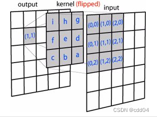
卷积核:也称为过滤器,就是图像处理时,给定输入图像,输入图像中一个小区域中像素加权平均后成为输出图像中的每个对应像素,其中权值由一个函数定义,这个函数称为卷积核。CNN 中的卷积核跟传统的卷积核本质没有什么不同。仍然以图像为例,卷积核依次与输入不同位置的图像块做卷积,得到输出。
特征图:在每个卷积层,数据都是以三维形式存在的。你可以把它看成许多个二维图片叠在一起,其中每一个称为一个feature map。在输入层,如果是灰度图片,那就只有一个feature map;如果是彩色图片,一般就是3个feature map(红绿蓝)。层与层之间会有若干个卷积核(kernel),上一层和每个feature map跟每个卷积核做卷积,都会产生下一层的一个feature map。
特征选择:是指从已有的M个特征(Feature)中选择N个特征使得系统的特定指标最优化,是从原始特征中选择出一些最有效特征以降低数据集维度的过程。CNN中采样层负责特征选择。
步长:即每次运算的时候卷积核移动的量。
填充:在原矩阵边界中添加一些值避免信息损失。
感受野:简单来说就是卷积神经网络中每层的卷积特征图上的像素点在原始图像中映射的区域大小,也就相当于高层的特征图中的像素点受原图多大区域的影响。
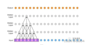
如图是三层的神经卷积神经网络,每一层卷积核的kernel_size=3, stride=1,那么最上层特征所对应的感受野就为如图所示紫色区域的7x7。
二、探究不同卷积核的作用
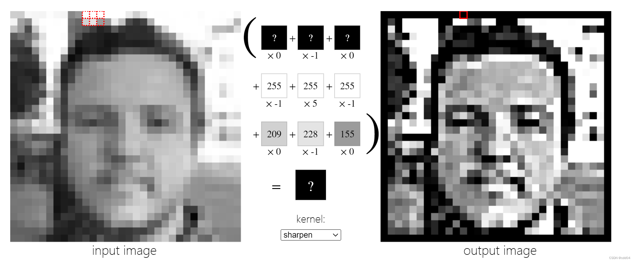
1.锐化
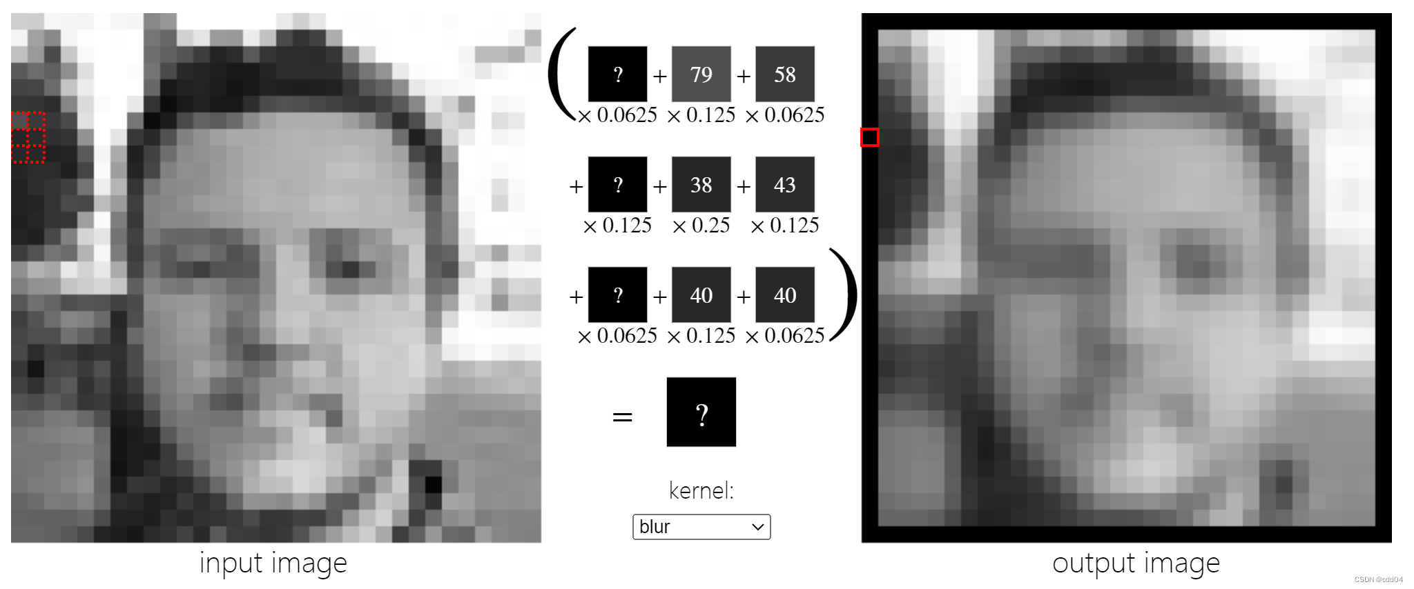
2.模糊
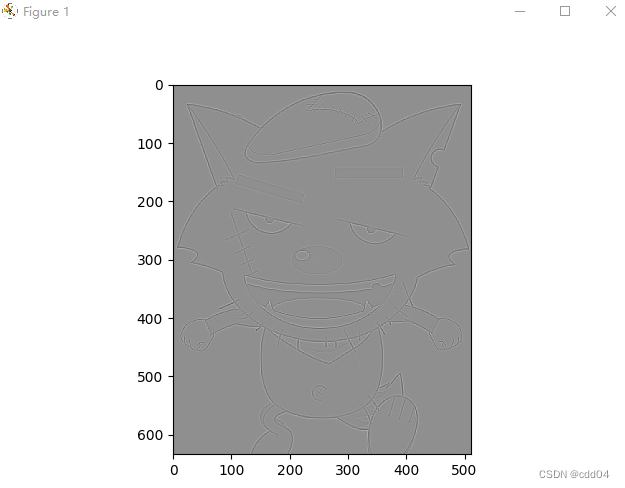
3. 浮雕:提取边界并调换颜色。
 参考:Image Kernels explained visually (setosa.io)
三、编程实现
1.实现灰度图的边缘检测、锐化、模糊。(必做)
边缘检测:
import numpy as np
import torch
from torch import nn
from torch.autograd import Variable
from PIL import Image
import matplotlib.pyplot as plt
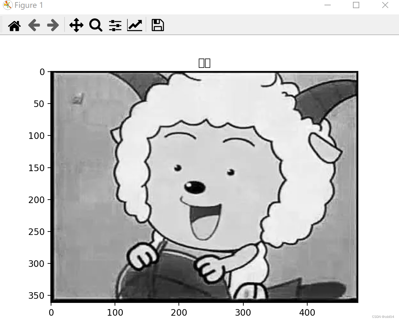
im = Image.open('1.png').convert('L') # 读入一张灰度图的图片
im = np.array(im, dtype='float32') # 将其转换为一个矩阵
print(im.shape[0], im.shape[1])
plt.imshow(im.astype('uint8'), cmap='gray') # 可视化图片
plt.title('原图')
plt.show()
im = torch.from_numpy(im.reshape((1, 1, im.shape[0], im.shape[1])))
conv1 = nn.Conv2d(1, 1, 3, bias=False) # 定义卷积
sobel_kernel = np.array([[-1, -1, -1],
[-1, 8, -1],
[-1, -1, -1]], dtype='float32') # 定义轮廓检测算子
sobel_kernel = sobel_kernel.reshape((1, 1, 3, 3)) # 适配卷积的输入输出
conv1.weight.data = torch.from_numpy(sobel_kernel) # 给卷积的 kernel 赋值
edge1 = conv1(Variable(im)) # 作用在图片上
x = edge1.data.squeeze().numpy()
print(x.shape) # 输出大小
plt.imshow(x, cmap='gray')
plt.show()
锐化:
import matplotlib.pyplot as plt
import numpy as np
import cv2 as cv


# 求卷积运算
def convolution(img_old, kernel):
    img_new = np.zeros(img.shape, dtype=int)
    for i in range(1, img_new.shape[0] - 1):  # 第一列和最后一列不用处理
        for j in range(1, img_new.shape[1] - 1):
            tmp = 0  # 初始化为0,用来求和
            for k in range(-1, 2):
                for l in range(-1, 2):
                    tmp += img_old[i + k][j + l] * kernel[k + 1][l + 1]
            img_new[i][j] = abs(tmp)
    return img_new


plt.rc("font", family='Microsoft YaHei')
img = plt.imread('1.png')  # 读取图片
img = img[:, :, 0]  # 把图片从三通道变为单通道
plt.subplot(241), plt.title("1.原图"), plt.axis('off')
plt.imshow(img, cmap="gray")

#  水平锐化
kernel_horizontal = np.array([[1, 2, 1],
                              [0, 0, 0],
                              [-1, -2, -1]])
img_horizontal = convolution(img, kernel_horizontal)
plt.subplot(242), plt.title("2.水平锐化后"), plt.axis('off')
plt.imshow(img_horizontal, cmap="gray")
# 垂直锐化

kernel_vertical = np.array([[1, 0, -1],
                            [2, 0, -2],
                            [1, 0, -1]])
img_vertical = convolution(img, kernel_vertical)
plt.subplot(243), plt.title("3.垂直锐化后"), plt.axis('off')
plt.imshow(img_vertical, cmap="gray")
plt.show()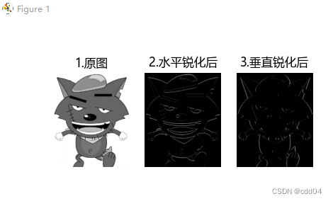
模糊:
import cv2
import numpy as np

img = cv2.imread("1.png")
kernel = np.ones((5,5),np.uint8)

imgGray = cv2.cvtColor(img,cv2.COLOR_BGR2GRAY)
imgBlur = cv2.GaussianBlur(imgGray,(7,7),0)

cv2.imshow("Gaussian Blur",imgBlur)
cv2.waitKey(0)
2.调整卷积核参数,测试并总结。(必做)
增加步长为3:
conv1 = nn.Conv2d(1, 1, 3,stride=3, bias=False) # 定义卷积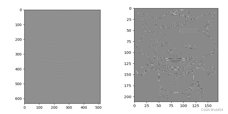
可以看出增加步长使图像更加模糊。
增加padding为6:
conv1 = nn.Conv2d(1, 1, 3,padding=6, bias=False) # 定义卷积
3.使用不同尺寸图片,测试并总结。(必做)
原图:
边缘检测: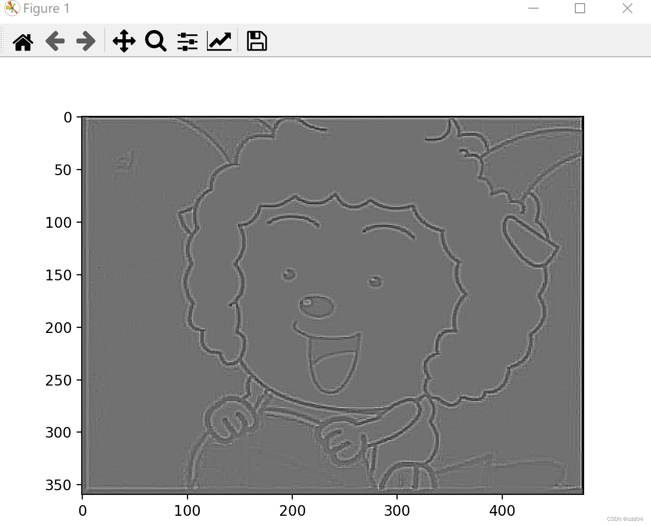
锐化:

模糊:

总结
通过本次实验对卷积操作和图像的本质有了更深的理解,在卷积神经网络面前,所有图像都是矩阵,矩阵中就是一个个的像素,这些像素组成了我们肉眼看到的图像。从信号与系统的角度看,卷积很多时候出现在一个系统的单位脉冲响应与输入信号上,用于求出系统在一定输入下所对应的输出。神经网络的多层结构从一开始的设想是模仿生物的神经元的一层一层传递的结构,从一开始的神经元判断角和边等等到大的局部特征最终得到所看到的目标是否是与神经元中记忆的某一个模式所匹配来进行目标的判断。


 683
683


 被折叠的 条评论
为什么被折叠?
被折叠的 条评论
为什么被折叠?
 到【灌水乐园】发言


