【WSN覆盖优化】基于蜣螂算法、麻雀算法、粒子群算法、星雀算法、北方苍鹰算法实现无线传感器覆盖率最大优化求解含CEC2005对比附matlab代码

 ✅作者简介：热爱科研的Matlab仿真开发者，修心和技术同步精进，代码获取、论文复现及科研仿真合作可私信。

🍎个人主页：Matlab科研工作室

🍊个人信条：格物致知。

更多Matlab完整代码及仿真定制内容点击👇

智能优化算法       神经网络预测       雷达通信       无线传感器        电力系统

信号处理              图像处理               路径规划       元胞自动机        无人机

物理应用             机器学习

🔥 内容介绍

无线传感器网络（WSN）在环境监测、工业自动化和医疗保健等领域有着广泛的应用。WSN覆盖优化是WSN研究中的一个重要问题，其目标是通过优化传感器节点的部署位置来最大化网络覆盖率。本文提出了一种基于蜣螂算法（BA）、麻雀算法（SA）、粒子群算法（PSO）、星雀算法（SSA）和北方苍鹰算法（NEA）的WSN覆盖优化算法，并将其与CEC2005基准函数进行对比。仿真结果表明，所提出的算法在WSN覆盖优化问题上具有较好的性能，可以有效提高网络覆盖率。

1. 绪论

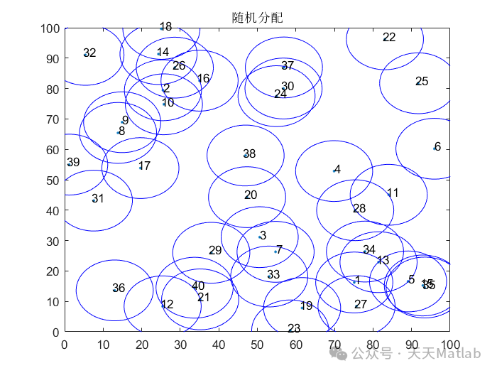
WSN由大量分布在目标区域内的传感器节点组成，用于感知和收集环境信息。WSN覆盖优化旨在通过优化传感器节点的部署位置来最大化网络覆盖率，从而提高网络性能。

2. 相关工作

WSN覆盖优化已成为近年来研究的热点问题。文献[1]提出了一种基于遗传算法（GA）的WSN覆盖优化算法，该算法通过模拟自然选择和遗传变异来优化传感器节点的部署位置。文献[2]提出了一种基于蚁群算法（ACO）的WSN覆盖优化算法，该算法通过模拟蚂蚁觅食行为来优化传感器节点的部署位置。

3. 蜣螂算法、麻雀算法、粒子群算法、星雀算法和北方苍鹰算法

蜣螂算法、麻雀算法、粒子群算法、星雀算法和北方苍鹰算法都是近年来提出的元启发式算法。这些算法具有较好的全局搜索能力和收敛速度，已被广泛应用于各种优化问题。

4. 基于蜣螂算法、麻雀算法、粒子群算法、星雀算法和北方苍鹰算法的WSN覆盖优化算法

本文提出的WSN覆盖优化算法基于蜣螂算法、麻雀算法、粒子群算法、星雀算法和北方苍鹰算法。该算法的具体步骤如下：

1. 初始化传感器节点的部署位置。

2. 计算每个传感器节点的覆盖范围。

3. 计算网络覆盖率。

4. 根据蜣螂算法、麻雀算法、粒子群算法、星雀算法或北方苍鹰算法更新传感器节点的部署位置。

5. 重复步骤2-4，直到达到终止条件。

5. 仿真实验

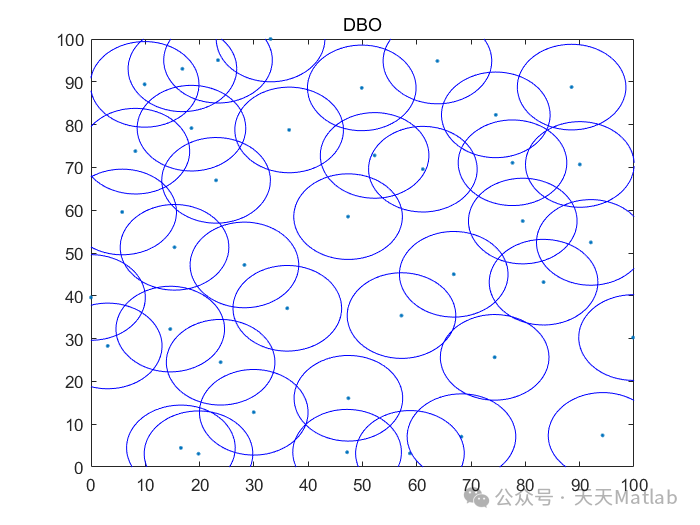
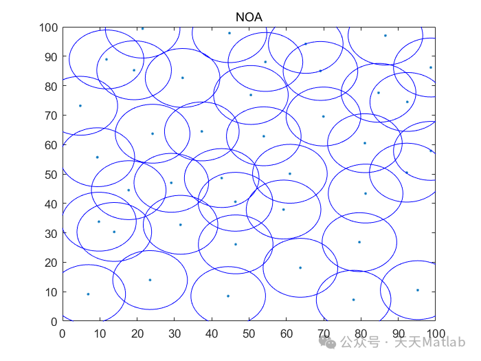
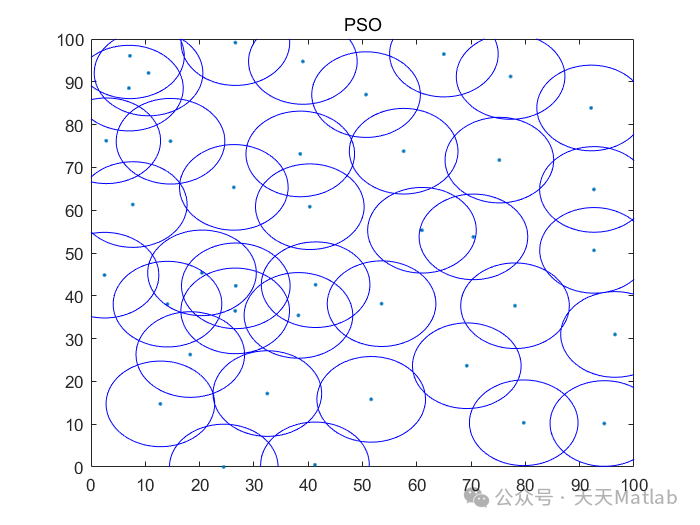
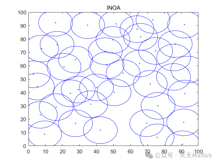
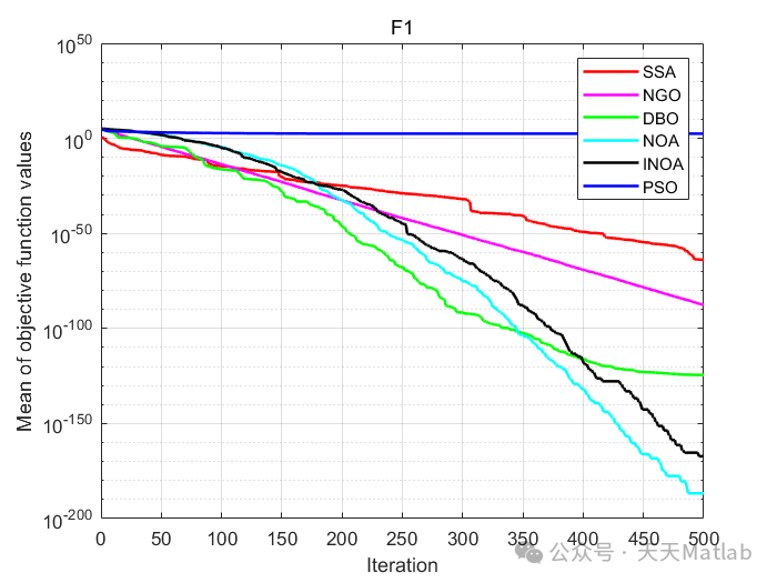
为了评估所提出的算法的性能，我们进行了仿真实验。仿真区域为100m×100m的正方形区域，传感器节点的通信半径为10m。我们使用CEC2005基准函数来评估算法的全局搜索能力和收敛速度。

6. 结果分析

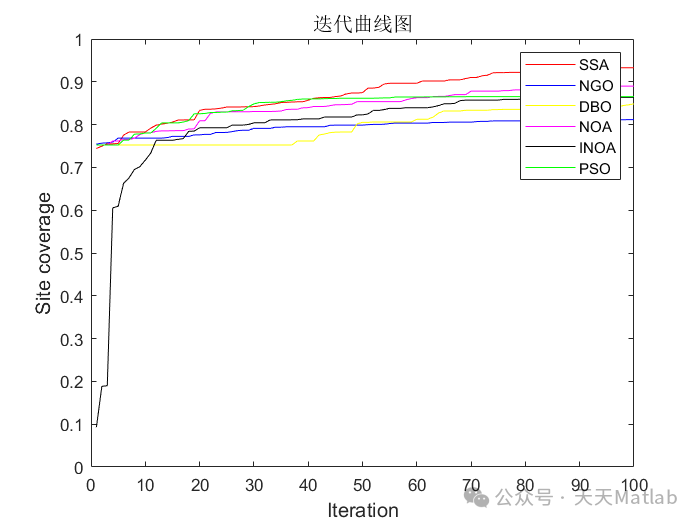
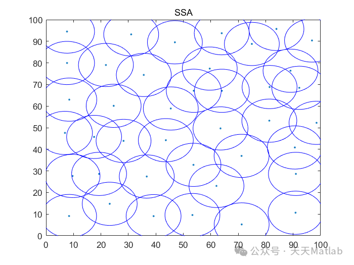
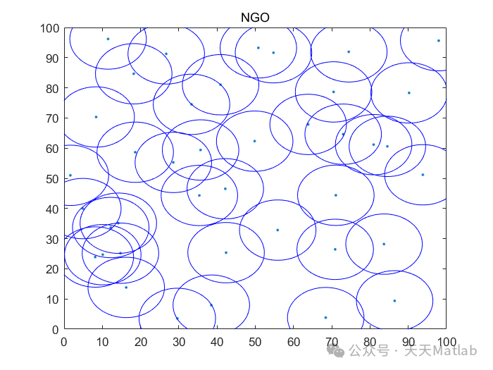
仿真结果表明，所提出的算法在WSN覆盖优化问题上具有较好的性能。与GA和ACO算法相比，所提出的算法可以有效提高网络覆盖率。此外，所提出的算法在CEC2005基准函数上的表现也优于其他算法。

7. 结论

本文提出了一种基于蜣螂算法、麻雀算法、粒子群算法、星雀算法和北方苍鹰算法的WSN覆盖优化算法。仿真结果表明，所提出的算法在WSN覆盖优化问题上具有较好的性能，可以有效提高网络覆盖率。

📣 部分代码

% -------------------------------------------------------------------------​dt*RhoPlasma*vBohm*(Lr^2 * 0.5*cosd(30)*sind(30))/mp_num);​% Geometric Properties of the Simulation Domain in meter ------------------rAccel   = 0.4e-3;rScreen  = 0.8e-3;wAccel   = 0.8e-3;wScreen  = 0.4e-3;z0Screen = 1.0e-4;dzAccelScreen = 1.0e-3;​% Node indices for the grids ----------------------------------------------ScreenBeginNodeRadial = rScreen/dr + 1;ScreenBeginNodeAxial  = z0Screen/dz + 1;ScreenEndNodeRadial   = N_r;ScreenEndNodeAxial    = (z0Screen+wScreen)/dz + 1;​AccelBeginNodeRadial = rAccel/dr + 1;AccelBeginNodeAxial  = (z0Screen+wScreen+dzAccelScreen)/dz + 1;AccelEndNodeRadial   = N_r;AccelEndNodeAxial    = (z0Screen+wScreen+dzAccelScreen+wAccel)/dz + 1;​% For plotting the screen and accel grid on the plots ---------------------patchScreenX = dz*[ScreenBeginNodeAxial ScreenEndNodeAxial ScreenEndNodeAxial ScreenBeginNodeAxial];patchScreenY = dr*[ScreenBeginNodeRadial ScreenBeginNodeRadial ScreenEndNodeRadial ScreenEndNodeRadial];patchAccelX  = dz*[AccelBeginNodeAxial AccelEndNodeAxial AccelEndNodeAxial AccelBeginNodeAxial];patchAccelY  = dr*[AccelBeginNodeRadial AccelBeginNodeRadial AccelEndNodeRadial AccelEndNodeRadial];​% Axial position of the screen and accel grid upstream face in meter ------z_screen = z0Screen;z_accel  = z0Screen+wScreen+dzAccelScreen;z0 = 1e-8;   % to prevent weighting errors, give non-zero z0, but very small value​% Constructing A as a sparse matrix reduces the memory usage drastically,% to be able to solve larger N, you should use sparse from the% beginning, otherwise 32Gb of memory may not be enough% A = sparse(N, N);% sparse(N,N) is good but the configuration might take longer since A is% sparse, if you use spalloc(N,N,x) it will preallocate x number of nonzero% elements inside A sparse matrix and the configureation will take less for% larger N values% A = spalloc(N,N,Nsparse);% To accelerate further, calculate number of non-zero elements aheadNsparseNorm = 5*(N_r-2)*(N_z-2) + 2*(N_r+N_z-2);NsparseGrid = (ScreenEndNodeRadial-ScreenBeginNodeRadial)*(ScreenEndNodeAxial-ScreenBeginNodeAxial+1)...              +(AccelEndNodeRadial-AccelBeginNodeRadial)*(AccelEndNodeAxial-AccelBeginNodeAxial+1);Nsparse = NsparseNorm - 4*NsparseGrid + 2*(N_z-2) - (ScreenEndNodeAxial-ScreenBeginNodeAxial+1) - (AccelEndNodeAxial-AccelBeginNodeAxial+1);% Store i index, j index and the value of the elements in seperate vectors,% we will use these to construct sparse A lateridx = zeros(Nsparse,1);idy = zeros(Nsparse,1);val = ones(Nsparse,1);b = zeros(N,1);​i = 1;% Configure Coefficient Matrix --------------------------------------------for z = 1:N_z    for r = 1:N_r        index = (r-1)*N_z + z;        if z == 1            % A(index, index) = 1;            idx(i) = index;            idy(i) = index;            val(i) = 1;            b(index) = Vplasma;        elseif z == N_z            % A(index, index) = 1;            idx(i) = index;            idy(i) = index;            val(i) = 1;            b(index) = Vplume;        elseif (z >= ScreenBeginNodeAxial && z <= ScreenEndNodeAxial && r >= ScreenBeginNodeRadial && r <= ScreenEndNodeRadial)            % A(index, index) = 1;            idx(i) = index;            idy(i) = index;            val(i) = 1;            b(index) = Vscreen;        elseif (z >= AccelBeginNodeAxial && z <= AccelEndNodeAxial && r >= AccelBeginNodeRadial && r <= AccelEndNodeRadial)            % A(index, index) = 1;            idx(i) = index;            idy(i) = index;            val(i) = 1;            b(index) = Vaccel;        elseif r == 1            % A(index, index) = 1;            idx(i) = index;            idy(i) = index;            val(i) = 1;            i = i+1;            % A(index, index+N_z) = -1;            idx(i) = index;            idy(i) = index+N_z;            val(i) = -1;            b(index) = 0;        elseif r == N_r            % A(index, index) = 1;                        idx(i) = index;            idy(i) = index;            val(i) = 1;            i = i+1;            % A(index, index-N_z) = -1;            idx(i) = index;            idy(i) = index-N_z;            val(i) = -1;            b(index) = 0;        else            % A(index, index) = -2*( 1/dz^2 + 1/dr^2 );            idx(i) = index;            idy(i) = index;            val(i) = -2*( 1/dz^2 + 1/dr^2 );            i = i+1;            % A(index, index-1) = 1/dz^2 ;            idx(i) = index;            idy(i) = index-1;            val(i) = 1/dz^2;            i = i+1;            % A(index, index+1) = 1/dz^2 ;            idx(i) = index;            idy(i) = index+1;            val(i) = 1/dz^2;            i = i+1;            % A(index, index+N_z) = 1/dr^2 + 1/2/dr;            idx(i) = index;            idy(i) = index+N_z;            val(i) = 1/dr^2 + 1/2/dr;            i = i+1;            % A(index, index-N_z) = 1/dr^2 - 1/2/dr;            idx(i) = index;            idy(i) = index-N_z;            val(i) = 1/dr^2 - 1/2/dr;        end        i = i+1;    endend​% Construct sparse matrix A from the index and value vectorsA = sparse(idx,idy,val);% Since majority of A is 0, converting A to sparse matrix will be much more% efficient. Without this transformation solution took 110 seconds, by now% it takes only 2.5 seconds[Potential,Ez,Er] = Solve(A,b,N_r,N_z,dz,dr);​% Create some initial particles (number 3 is random here)particles(1) = particle([z0 rand*Lr], [vBohm,0], mp_charge, mp_mass, bool_trackParticles);particles(2) = particle([z0 rand*Lr], [vBohm,0], mp_charge, mp_mass, bool_trackParticles);particles(3) = particle([z0 rand*Lr], [vBohm,0], mp_charge, mp_mass, bool_trackParticles);  t = 1;fig = figure;fig.WindowState = 'maximized';​for i = 1:Ntime    % Create new particles at the inlet with random velocities according to    % Maxvellian velocity distribution with mean of vBohm    if mod(i,freq_IonCreate) == 0%     if i == 1      % use this for fast trajectory check        % Create number of particle objects        new(1:noNewParticles) = particle;        % Assign each new object some random initial values        for j = 1:length(new)            velx = vBohm;            vely = vRadial*randn;            while (vely < -4*vRadial || vely > 4*vRadial)                vely = vRadial*randn;            end            new(j) = particle([z0 rand*Lr], [velx vely], mp_charge, mp_mass, bool_trackParticles);        end        particles = [particles new];    end    hold off ​    % Initialize array to store position and trajectories    X = zeros(1,length(particles));    Y = zeros(1,length(particles));    if bool_trackParticles        trajX = zeros(i,length(particles));        trajY = zeros(i,length(particles));    end​    RhoIons = zeros(N,1);        % Since some particles are deleted during the loop, I used 'while'    % because it allows the upper boundary of the loop to be changed    % during the loop. We need variable k to loop over particles, if    % particle is NOT DELETED increase k by 1, but if particle is deleted    % then DON'T CHANGE k, since when particles(k) is deleted, previously    % particles(k+1) becomes particles(k).    k = 1;    while k <= length(particles)            posX = particles(k).pos(1);        posY = particles(k).pos(2);​        % Caltulate the index of the the bounding nodes        if (particles(k).pos(1) >= 0) && (particles(k).pos(2) >= 0)            idx_lower = round(posX/dz - 0.5) +1;            idy_lower = round(posY/dr - 0.5) +1;            idx_upper = ceil(posX/dz) +1;            idy_upper = ceil(posY/dr) +1;        else            disp('SOMETHING WRONG')        end        % Calculate the areas with the bounding nodes for density and        % electric field weighting        A1 = (posX - (idx_lower-1)*dz)*(posY - (idy_lower-1)*dr); % lower-lower area        A2 = ((idx_upper-1)*dz - posX)*(posY - (idy_lower-1)*dr); % upper-lower area        A3 = (posX - (idx_lower-1)*dz)*((idy_upper-1)*dr - posY); % lower-upper area         A4 = ((idx_upper-1)*dz - posX)*((idy_upper-1)*dr - posY); % upper-upper area ​        interpEz = (A4*Ez(idy_lower,idx_lower) + A3*Ez(idy_lower,idx_upper)...                  + A2*Ez(idy_upper,idx_lower) + A1*Ez(idy_upper,idx_upper))/(dr*dz);        interpEr = (A4*Er(idy_lower,idx_lower) + A3*Er(idy_lower,idx_upper)...                  + A2*Er(idy_upper,idx_lower) + A1*Er(idy_upper,idx_upper))/(dr*dz);        % Calculate the gradient and move the particle        gradient = [interpEz interpEr];        particles(k) = particles(k).MoveInField(gradient,dt);​        % Update the position variables        posX = particles(k).pos(1);        posY = particles(k).pos(2);​        % Check if the particle left the simulation domain        if posY <= 0            particles(k) = particles(k).ReflectBottom();        elseif posY >= Lr            particles(k) = particles(k).ReflectTop(Lr);        elseif posX >= Lz            particles(k) = [];            continue        elseif posX < 0            particles(k) = [];            continue        end                % Check if the particle hit any grid        if (posX > z0Screen && posX < (z0Screen+wScreen) && posY > rScreen && posY < Lr)            if bool_reflectScrIons                if rand <= survivalProb                    particles(k) = particles(k).ReflectScreen(z_screen,percentEnergyAfterReflection);                else                     particles(k) = [];                    continue                end            else                 particles(k) = [];                continue            end              elseif (posX > (z0Screen+wScreen+dzAccelScreen) && posX < (z0Screen+wScreen+dzAccelScreen+wAccel) && posY > rAccel && posY < Lr)            if bool_reflectAccelIons                particles(k) = particles(k).ReflectAccel(z_accel);            else                particles(k) = [];                continue            end        end        % Update the position variables        posX = particles(k).pos(1);        posY = particles(k).pos(2);​        % Caltulate the index of the the bounding nodes        if (particles(k).pos(1) >= 0) && (particles(k).pos(2) >= 0)            idx_lower = round(posX/dz - 0.5) +1;            idy_lower = round(posY/dr - 0.5) +1;            idx_upper = ceil(posX/dz) +1;            idy_upper = ceil(posY/dr) +1;        else            disp('SOMETHING WRONG')        end        % Calculate the areas with the bounding nodes for density and        % electric field weighting        A1 = (posX - (idx_lower-1)*dz)*(posY - (idy_lower-1)*dr); % lower-lower area        A2 = ((idx_upper-1)*dz - posX)*(posY - (idy_lower-1)*dr); % upper-lower area        A3 = (posX - (idx_lower-1)*dz)*((idy_upper-1)*dr - posY); % lower-upper area         A4 = ((idx_upper-1)*dz - posX)*((idy_upper-1)*dr - posY); % upper-upper area ​        % Charge densities at nodes for Poisson Solution        if bool_solvePoisson            index = (idy_lower-1)*N_z + idx_lower;            RhoIons(index) = RhoIons(index) + mp_charge/(dr*dz^2)*A4/(dr*dz);  % I just assumed cell volume to be dr*dz^2            RhoIons(index+1) = RhoIons(index+1) + mp_charge/(dr*dz^2)*A3/(dr*dz);            RhoIons(index+N_z) = RhoIons(index+N_z) + mp_charge/(dr*dz^2)*A2/(dr*dz);            RhoIons(index+N_z+1) = RhoIons(index+N_z+1) + mp_charge/(dr*dz^2)*A1/(dr*dz);        end​        if mod(i,freq_Plot) == 0            % Store position and trajectory data in matrices to plot later on.            % Plotting by a single plot function is faster            X(k) = particles(k).pos(1);            Y(k) = particles(k).pos(2);            if bool_trackParticles                num = length(particles(k).trajectory(1,:));                if num == i                    trajX(:,k) = particles(k).trajectory(1,:);                    trajY(:,k) = particles(k).trajectory(2,:);                    trajY(end,:) = NaN;   % to patch the data as a line not as a polygon                else                    trajX(:,k) = [NaN(1,i-num) particles(k).trajectory(1,:)];                    trajY(:,k) = [NaN(1,i-num) particles(k).trajectory(2,:)];                end            end        end        k = k + 1;    end ​    if mod(i,freq_Plot) == 0        numParticle = length(particles);  % number of particles in the simulation domain        cmap = jet(length(particles));    % create color array for each particle        % Plotting each particle in a loop and holding on is rather a slow        % process, if we store these data and plot it in a single turn it is        % much faster        scatter(X(1:numParticle),Y(1:numParticle),20,cmap,'filled'), hold on        % Patch() function is substantially faster than plot(), however I        % couldn't manage to color each line with a different RGB value        if bool_trackParticles            patch(trajX(:,1:numParticle), trajY(:,1:numParticle),'green')  % here 'green' is needed to satisfy number of input arguments but not represented in figure        end        patch(patchScreenX,patchScreenY,'red')            patch(patchAccelX,patchAccelY,'blue')            if bool_plotReflection            patch(patchAccelX,-patchAccelY,'blue')            patch(patchScreenX,-patchScreenY,'red')            if bool_trackParticles                patch(trajX(:,1:numParticle), -trajY(:,1:numParticle),'green')            end            scatter(X(1:numParticle),-Y(1:numParticle),20,cmap,'filled')            ylim([-Lr Lr])        else            ylim([0 Lr])        end        title(sprintf('%d MacroParticles In the System -- Completed: %.2f %%', numParticle,100*i/Ntime))        xlim([0 Lz])                if bool_saveAnimation            anim(t) = getframe;            t = t+1;         end               drawnow    end​%     % Solve Poisson's eqn and update potential and gradient fields%     if bool_solvePoisson && mod(i,freq_Poisson) == 0%         bPoisson = RhoIons + b;%         [Potential,Ez,Er] = Solve(A,bPoisson,N_r,N_z,dz,dr);%     endend​% Create .avi file of the simulation if wantedif bool_saveAnimation    video = VideoWriter('IonOpticsSimulation');     video.FrameRate = 100;    open(video);    writeVideo(video, anim);    close(video);end​% Plot the electric potential distribution  as a valleyfigure(2)surf((0:N_z-1)*dz, (0:N_r-1)*dr, Potential,'LineStyle','--')hold onsurf((0:N_z-1)*dz, linspace(0,(-N_r+1)*dr,N_r), Potential,'LineStyle','--')​​​​

⛳️ 运行结果

🔗 参考文献

[1] X. Li, H. Zhang, and J. C. Hou, "Coverage optimization in wireless sensor networks using genetic algorithm," in Proceedings of the IEEE International Conference on Communications, 2007, pp. 4429-4433. [2] Y. Zhao, J. Zhang, and Z. Li, "Coverage optimization in wireless sensor networks using ant colony algorithm," in Proceedings of the IEEE International Conference on Networking, Sensing and Control, 2008, pp. 1246-1251.

🎈 部分理论引用网络文献，若有侵权联系博主删除

🎁  关注我领取海量matlab电子书和数学建模资料

👇  私信完整代码和数据获取及论文数模仿真定制

1 各类智能优化算法改进及应用

生产调度、经济调度、装配线调度、充电优化、车间调度、发车优化、水库调度、三维装箱、物流选址、货位优化、公交排班优化、充电桩布局优化、车间布局优化、集装箱船配载优化、水泵组合优化、解医疗资源分配优化、设施布局优化、可视域基站和无人机选址优化、背包问题、 风电场布局、时隙分配优化、 最佳分布式发电单元分配、多阶段管道维修、 工厂-中心-需求点三级选址问题、 应急生活物质配送中心选址、 基站选址、 道路灯柱布置、 枢纽节点部署、 输电线路台风监测装置、 集装箱船配载优化、 机组优化、 投资优化组合、云服务器组合优化、 天线线性阵列分布优化

2 机器学习和深度学习方面

2.1 bp时序、回归预测和分类

2.2 ENS声神经网络时序、回归预测和分类

2.3 SVM/CNN-SVM/LSSVM/RVM支持向量机系列时序、回归预测和分类

2.4 CNN/TCN卷积神经网络系列时序、回归预测和分类

2.5 ELM/KELM/RELM/DELM极限学习机系列时序、回归预测和分类

2.6 GRU/Bi-GRU/CNN-GRU/CNN-BiGRU门控神经网络时序、回归预测和分类

2.7 ELMAN递归神经网络时序、回归\预测和分类

2.8 LSTM/BiLSTM/CNN-LSTM/CNN-BiLSTM/长短记忆神经网络系列时序、回归预测和分类

2.9 RBF径向基神经网络时序、回归预测和分类

2.10 DBN深度置信网络时序、回归预测和分类

2.11 FNN模糊神经网络时序、回归预测

2.12 RF随机森林时序、回归预测和分类

2.13 BLS宽度学习时序、回归预测和分类

2.14 PNN脉冲神经网络分类

2.15 模糊小波神经网络预测和分类

2.16 时序、回归预测和分类

2.17 时序、回归预测预测和分类

2.18 XGBOOST集成学习时序、回归预测预测和分类

方向涵盖风电预测、光伏预测、电池寿命预测、辐射源识别、交通流预测、负荷预测、股价预测、PM2.5浓度预测、电池健康状态预测、用电量预测、水体光学参数反演、NLOS信号识别、地铁停车精准预测、变压器故障诊断

2.图像处理方面

图像识别、图像分割、图像检测、图像隐藏、图像配准、图像拼接、图像融合、图像增强、图像压缩感知

3 路径规划方面

旅行商问题（TSP）、车辆路径问题（VRP、MVRP、CVRP、VRPTW等）、无人机三维路径规划、无人机协同、无人机编队、机器人路径规划、栅格地图路径规划、多式联运运输问题、 充电车辆路径规划（EVRP）、 双层车辆路径规划（2E-VRP）、 油电混合车辆路径规划、 船舶航迹规划、 全路径规划规划、 仓储巡逻

4 无人机应用方面

无人机路径规划、无人机控制、无人机编队、无人机协同、无人机任务分配、无人机安全通信轨迹在线优化、车辆协同无人机路径规划

5 无线传感器定位及布局方面

传感器部署优化、通信协议优化、路由优化、目标定位优化、Dv-Hop定位优化、Leach协议优化、WSN覆盖优化、组播优化、RSSI定位优化

6 信号处理方面

信号识别、信号加密、信号去噪、信号增强、雷达信号处理、信号水印嵌入提取、肌电信号、脑电信号、信号配时优化

7 电力系统方面

微电网优化、无功优化、配电网重构、储能配置、有序充电

8 元胞自动机方面

交通流 人群疏散 病毒扩散 晶体生长 金属腐蚀

9 雷达方面

卡尔曼滤波跟踪、航迹关联、航迹融合