最大协方差（Maximum covarivance analysis，MCA）

最大协方差分析(MCA)是气候和气象学领域中的一种奇异值分解(SVD)分析，已被广泛应用于探测两个时间序列之间变化的耦合模态。MCA构造了两个数据集之间的协方差矩阵，然后对得到的矩阵进行SVD。

MCA之间的时间协方差最大化两个不同的数据字段和密切相关主成分分析(PCA) /经验正交函数(EOF分析)分析。虽然EOF分析最大化方差在单个数据字段,MCA允许提取的主导模式之间的共变两个不同的数据字段。当两个输入字段相同,MCA降低到标准EOF分析。

公式：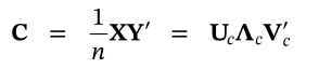

在这里介绍一个py包xmac：该软件包的目的是为气候科学界提供一种灵活的工具，以简单且一致的方式执行最大协方差分析 (MCA)。鉴于 xarray 在气候科学界的广泛流行，xmca 支持 xarray.DataArray 以及 numpy.ndarray 作为输入格式。

py包的安装

pip install xmca

导入包

from xmca.array import MCA  # use with np.ndarray
from xmca.xarray import xMCA  # use with xr.DataArray

例如，我们以 xarray 附带的北美表面温度为例。注意：仅适用于 xr.DataArray，不适用于 xr.Dataset。

import xarray as xr  # only needed to obtain test data

# split data arbitrarily into west and east coast
data = xr.tutorial.open_dataset('air_temperature').air
west = data.sel(lon=slice(200, 260))
east = data.sel(lon=slice(260, 360))

PCA / EOF分析：构建一个只有一个字段的模型并对其进行求解以执行标准的 PCA/EOF 分析。

pca = xMCA(west)                        # PCA of west coast
pca.solve(complexify=False)            # True for complex PCA

svals = pca.singular_values()     # singular vales = eigenvalues for PCA
expvar      = pca.explained_variance()  # explained variance
pcs         = pca.pcs()                 # Principal component scores (PCs)
eofs        = pca.eofs()                # spatial patterns (EOFs)

通过选择要旋转的 EOF 数量 (n_rot) 以及 Promax 参数（功率）来旋转模型，可以获得 Varimax/Promax 旋转解。这里，power=1 等于 Varimax 旋转解。

pca.rotate(n_rot=10, power=1)

expvar_rot  = pca.explained_variance()  # explained variance
pcs_rot     = pca.pcs()                 # Principal component scores (PCs)
eofs_rot    = pca.eofs()                # spatial patterns (EOFs)

MCA：与 PCA/EOF 分析相同，但有两个输入字段而不是一个。

mca = xMCA(west, east)                  # MCA of field A and B
mca.solve(complexify=False)            # True for complex MCA

eigenvalues = mca.singular_values()     # singular vales
pcs = mca.pcs()                         # expansion coefficient (PCs)
eofs = mca.eofs()                       # spatial patterns (EOFs)

显著性分析:估计获得的模式的重要性的一种简单方法是运行基于不相关的高斯白噪声（称为规则 N）的蒙特卡罗模拟（Overland 和 Preisendorfer 1982）。在这里，我们创建了 200 个这样的合成数据集，并将合成数据与真实奇异光谱进行比较以评估重要性。

surr = mca.rule_n(200)
median = surr.median('run')
q99 = surr.quantile(.99, dim='run')
q01 = surr.quantile(.01, dim='run')

cutoff = np.sum((svals - q99 > 0)).values  # first 8 modes significant

fig = plt.figure(figsize=(10, 4))
ax = fig.add_subplot(111)
svals.plot(ax=ax, yscale='log', label='true')
median.plot(ax=ax, yscale='log', color='.5', label='rule N')
q99.plot(ax=ax, yscale='log', color='.5', ls=':')
q01.plot(ax=ax, yscale='log', color='.5', ls=':')
ax.axvline(cutoff + 0.5, ls=':')
ax.set_xlim(-2, 200)
ax.set_ylim(1e-1, 2.5e4)
ax.set_title('Significance based on Rule N')
ax.legend()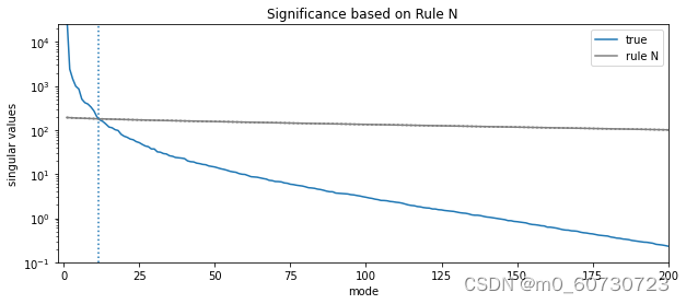

 

根据使用 200 次合成运行的规则 N，前 8 种模式是重要的。

保存和加载分析

mca.save_analysis('my_analysis')    # this will save the data and a respective
                                        # info file. The files will be stored in a
                                        # special directory
mca2 = xMCA()                       # create a new, empty instance
mca2.load_analysis('my_analysis/info.xmca') # analysis can be
                                        # loaded via specifying the path to the
                                        # info file created earlier

结果可视化

mca2.set_field_names('West', 'East')
pkwargs = {'orientation' : 'vertical'}
mca2.plot(mode=1, **pkwargs)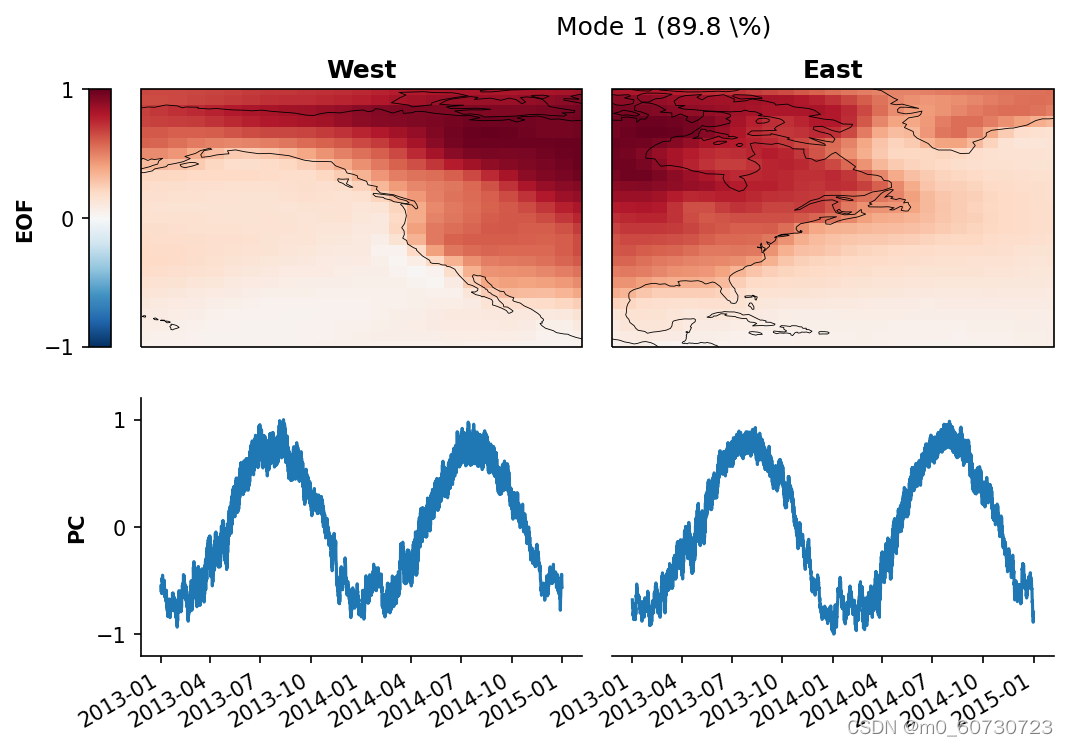

 在显示模式 1 的北美西海岸和东海岸的 T2m 上执行 MCA 后默认绘图方法的结果。

您可能想要修改绘图以获得更好的光学效果：

from cartopy.crs import EqualEarth  # for different map projections

# map projections for "left" and "right" field
projections = {
        'left': EqualEarth(),
        'right': EqualEarth()
}

pkwargs = {
        "figsize"     : (8, 5),
        "orientation" : 'vertical',
        'cmap_eof'    : 'BrBG',  # colormap amplitude
        "projection"  : projections,
}
mca2.plot(mode=3, **pkwargs)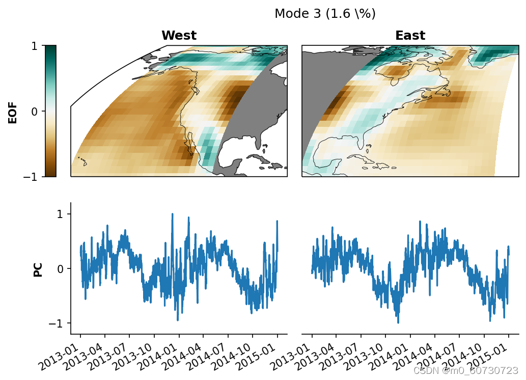

参考： 

Mo, R., 2003. Efficient algorithms for maximum covariance analysis of datasets with
many variables and fewer realizations: a revisit. J. Atmos. Ocean. Technol. 20,
1804–1809.

Niclas Rieger, 2021: nicrie/xmca: version x.y.z. doi:10.5281/zenodo.4749830.

欢迎关注VX公众号《遥感迷》，一起讨论学习