QPSK仿真系统MATLAB代码（超全！）

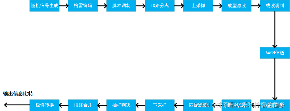
       实验流程就是按照上面的过程做的，还包含眼图、矢量图、星座图、误码率分析。所有代码全部手敲，注释是用英文写的，给大家分享一下，希望能够对大家有所帮助。

clc
clear all
close all

% Author: Mussy Max

%% Initializtion
symbol =1000; % numbers of symbols
bit = randi([0,1],1,2*symbol); % random bit
fc = 4e3; % carrier freq which determines how many carriers to represent
fs = 100e3; % sampling numbers of each pulse
sps = fs/(2*symbol); %samples of each pulse
T = 1; % time for each bit
figure(1);
subplot(2,1,1)
plot(bit);
title('raw bit');
time_delay = 0; % wether consodering the time delay of filter

%% GrayCode Pre-coding
Gray = [0,0;0,1;1,1;1,0];
bit_gray = [];
for i = 1:symbol
    dec = bit(2*i-1)*2+bit(2*i)+1;
    bit_gray(2*i-1) = Gray(dec,1);
    bit_gray(2*i) = Gray(dec,2);
end
bit_gray = 2*bit_gray-1;  % turn to NBRZ
subplot(2,1,2)
plot(bit_gray);
title('gray bit');

%% IQ separation
I_raw = [];Q_raw = [];
for i = 1:symbol
    I_raw(i) = bit_gray(2*i-1);
    Q_raw(i) = bit_gray(2*i);
end
figure(4); % draw constellation chart
subplot(1,2,1)
plot(I_raw,Q_raw,'*');xlabel('I');ylabel('Q')
axis([-2,2,-2,2]);
title('constellation chart of the transmitter')


figure(11); % draw constellation chart
subplot(1,2,1)
plot(I_raw,Q_raw);xlabel('I');ylabel('Q')
axis([-2,2,-2,2]);
title('vector chart of the transmitter')
%% design a pulse form filter
roff = 0.5;
cutoff_symbols = 6;
fir_rcos = rcosdesign(roff, cutoff_symbols, sps, "sqrt"); % define a rcos filter
N_fir = length(fir_rcos);

%% upsampling IQ and filtering
I_upsample = upsample(I_raw, sps);
Q_upsample = upsample(Q_raw, sps);
I=conv(I_upsample,fir_rcos,'same');                                 
N = length(I);
Q =conv(Q_upsample,fir_rcos,'same');

if time_delay ==1
    I = I((N_fir-1)/2+1:end); % considering the time delay
    Q = Q((N_fir-1)/2+1:end);
end
figure(12)
subplot(2,1,1)
I_upsample_freq = fftshift(abs(fft(I_upsample)));
plot(-symbol*sps/2:1:symbol*sps/2-1,I_upsample_freq);
title('Signal spectrum before form filtering');xlabel('f/Hz');ylabel('Amplitude');
subplot(2,1,2)
I_freq = fftshift(abs(fft(I)));
plot(-symbol*sps/2:1:symbol*sps/2-1,I_freq);
title('Signal spectrum after form filtering');xlabel('f/Hz');ylabel('Amplitude');

figure(2)
subplot(4,1,1)
plot(I_upsample)
title('raw I')
subplot(4,1,2)
plot(Q_upsample)
title('raw Q')
subplot(4,1,3)
plot(I)
title('I after form filtering')
subplot(4,1,4)
plot(Q)
title('Q after form filtering')

%% Modulation
t = 0:1/fs:T/2-1/fs;
I_carrier = cos(2*pi*2*fc*t);
Q_carrier = sin(2*pi*2*fc*t);
I_modulated = I.*I_carrier; % I-road
Q_modulated = Q.*Q_carrier; % Q-road
sig_qpsk = I_modulated-Q_modulated; % I-Q = QPSK
figure(3); % draw 
subplot(2,1,1)
plot(sig_qpsk); % draw
title('QPSK signal')
subplot(2,1,2)
freq_qpsk = fftshift(abs(fft(sig_qpsk)));
plot(-symbol*sps/2:1:symbol*sps/2-1,freq_qpsk);
title('Spectrum of QPSK')


%% Channel Propagation
snr = 10;
sig_qpsk_received = awgn(sig_qpsk,snr,'measured');
figure(5);
subplot(2,1,1)
plot(sig_qpsk_received);
title('QPSK signal with awgn')
subplot(2,1,2)
freq_qpsk_received = fftshift(abs(fft(sig_qpsk_received)));
plot(-symbol*sps/2:1:symbol*sps/2-1,freq_qpsk_received );
title('Spectrum of QPSK with awgn')

%% Demodulation
I_demod = sig_qpsk_received.*I_carrier; % Coherent demodulation of I-road
Q_demod = -sig_qpsk_received.*Q_carrier; % Coherent demodulation of Q-road % watching the '-'
fir1_1=128;
lpf = fir1(fir1_1, 0.2); % design a low pass filter with hamming window
N_lpf = length(lpf);
I_lpf = filtfilt(lpf, 1, I_demod);
Q_lpf = filtfilt(lpf, 1, Q_demod);
if time_delay == 1
    I_lpf = I_lpf((N_lpl-1)/2+1:end); % considering the time delay
    Q_lpf = Q_lpf((N_lpl-1)/2+1:end); 
end
figure(6)
subplot(4,1,1)
plot(I_lpf);title('I road after LPF')
subplot(4,1,3)
plot(Q_lpf);title('Q road after LPF')

%% Matched filtering
I_mf=conv(I_lpf,fir_rcos,'same');                             
Q_mf=conv(Q_lpf,fir_rcos,'same');
% I_mf = I_lpf;Q_mf = Q_lpf;
if time_delay == 1
    I_mf = I_mf((N_fir-1)/2+1:end); % considering the time delay
    Q_mf = Q_mf((N_fir-1)/2+1:end);
end
subplot(4,1,2)
plot(I_mf);title('I road after MF')
subplot(4,1,4)
plot(Q_mf);title('Q road after MF')


%% Eye Diagram
I_final = downsample(I_mf,sps); % downsample
Q_final = downsample(Q_mf,sps); % downsample
figure(15)
subplot(2,1,1)
plot(I_raw);title('Transimited I-road subgrade band signal');xlabel('code');ylabel('Amplitude');
subplot(2,1,2)
plot(I_final);title('Recieved I-road subgrade band signal');xlabel('code');ylabel('Amplitude');
figure(4) % draw constellation chart
subplot(1,2,2)
plot(I_final,Q_final,'*');xlabel('I');ylabel('Q')
axis([-2,2,-2,2]);
title('constellation chart of the receiver')


eye_num = 2;           % numbers of eye    
Ts=1/fs;
Ti=0:Ts:eye_num*sps*Ts-Ts; 
for k=0:100
     s_r_I=I_mf((k+eye_num)*sps+1:(k+eye_num)*sps+eye_num*sps);  
     s_r_Q=Q_mf((k+eye_num)*sps+1:(k+eye_num)*sps+eye_num*sps);
     s_t_I=I((k+eye_num)*sps+1:(k+eye_num)*sps+eye_num*sps);
     s_t_Q=Q((k+eye_num)*sps+1:(k+eye_num)*sps+eye_num*sps);
     drawnow;
     figure(10);
     subplot(221);plot(Ti,s_r_I,'linewidth',2);title('Receiver Eyediagram of I-Road');hold on;
     subplot(222);plot(Ti,s_r_Q,'linewidth',2);title('Receiver Eyediagram of Q-Road');hold on;
     subplot(223);plot(Ti,s_t_I,'linewidth',2);title('Transimitter Eyediagram of I-Road');hold on;
     subplot(224);plot(Ti,s_t_Q,'linewidth',2);title('Transimitter Eyediagram of I-Road');hold on;
end
hold off



figure(11)
subplot(1,2,2)
plot(I_final,Q_final);xlabel('I');ylabel('Q')
axis([-2,2,-2,2]);
title('vector chart of the receiver')

%% Sample decision 
for i = 1:length(I_final) % decision of I-road
    if I_final(i)>=0
        I_final(i) = 1;
    else
        I_final(i) = -1;
    end
end
for i = 1:length(Q_final) % decision of Q-road
    if Q_final(i)>=0
        Q_final(i) = 1;
    else
        Q_final(i) = -1;
    end
end

%% IQ combination
bit_received = [];
for i = 1:length(I_final)
    bit_received(2*i-1) = I_final(i);
    bit_received(2*i) = Q_final(i);
end
figure(8)
subplot(2,1,1)
plot(bit_received);title('bit receiver')
subplot(2,1,2)
plot(bit_gray);title('bit transmitter')

%% Calculate error
bit_error = 0;
for m = 1:length(bit_received)
    if (bit_received(m) ~= bit_gray(m))
        bit_error = bit_error+1;
    end
end
ber = bit_error/length(bit_received);

%% Error by SNR
EbN0 = -6 : 8;
snr_1= EbN0 - 10 * log10(0.5 * sps) ;
ber_1=[];
for i = 1 : length(snr_1)
    snr = snr_1(i);
    sig_qpsk_received = awgn(sig_qpsk,snr,'measured');
    I_demod = sig_qpsk_received.*I_carrier; % Coherent demodulation of I-road
    Q_demod = -sig_qpsk_received.*Q_carrier; % Coherent demodulation of Q-road % watching the '-'
    lpf = fir1(128, 0.2); % design a low pass filter with hamming window
    N_lpf = length(lpf);
    I_lpf = filtfilt(lpf, 1, I_demod);
    Q_lpf = filtfilt(lpf, 1, Q_demod);

    I_mf=conv(I_lpf,fir_rcos,'same');                                  
    Q_mf=conv(Q_lpf,fir_rcos,'same');

    I_final = downsample(I_mf,sps); % downsample
    Q_final = downsample(Q_mf,sps); % downsample

    for i = 1:length(I_final) % decision of I-road
        if I_final(i)>=0
            I_final(i) = 1;
        else
            I_final(i) = -1;
        end
    end
    for i = 1:length(Q_final) % decision of Q-road
        if Q_final(i)>=0
            Q_final(i) = 1;
        else
            Q_final(i) = -1;
        end
    end

    bit_received = [];
    for i = 1:length(I_final)
        bit_received(2*i-1) = I_final(i);
        bit_received(2*i) = Q_final(i);
    end

    bit_error = 0;
    for m = 1:length(bit_received)
        if (bit_received(m) ~= bit_gray(m))
            bit_error = bit_error+1;
        end
    end
    ber = bit_error/length(bit_received);
    ber_1=[ber_1 ber];
end
ber_qpsk = berawgn(EbN0, 'psk', 4, 'nodiff');
figure(9)
semilogy(snr_1,ber_1 ,'-*', snr_1, ber_qpsk, '-+');
legend('experimental QPSK','theoretical QPSK');
xlabel('SNR');
ylabel('BER');
title('Simulation curve of bit error rate under different SNR');
legend('experimental curve','theoretical curve');