机器学习学习记录4：基于鸢尾花数据集的svm（求acc，可视化）问题

本次题目是

 

经历了数个小时的修改，过程省略

参考了两篇文章进行修改

(8条消息) 机器学习--支持向量机(sklearn)_想成为风筝的博客-CSDN博客_sklearn支持向量机

(8条消息) 基于sklearn的软硬间隔以及各类核函数的SVM实现_孑渡的博客-CSDN博客

获得以下代码：

import matplotlib.pyplot as plt
import matplotlib
import numpy as np
from sklearn import datasets, linear_model, model_selection, svm
from sklearn import datasets
from sklearn import svm
from sklearn.pipeline import Pipeline
from sklearn.preprocessing import StandardScaler
from sklearn.metrics import accuracy_score
from sklearn.model_selection import train_test_split

iris=datasets.load_iris()
X = iris["data"][:,(2,3)]
y = iris["target"]
y = np.array([1 if i == 1 else -1 for i in y])
xtrain, xtest, ytrain, ytest = train_test_split(X,y)
linear_svm = svm.LinearSVC(C=1)
linear_svm.fit(xtrain, ytrain)
y_pred = linear_svm.predict(xtest)
print('软间隔线性svm的准确率为：{}'.format(accuracy_score(ytest,y_pred)))
gauss_svm = svm.SVC(C=1, kernel='rbf')
gauss_svm.fit(xtrain, ytrain)
y_pred2 = gauss_svm.predict(xtest)
print('软间隔高斯核svm的准确率: %s' % (accuracy_score(ytest,y_pred2)))
linear_svm1 = svm.LinearSVC(C=100000)
linear_svm1.fit(xtrain, ytrain)
y_pred3 = linear_svm1.predict(xtest)
print('硬间隔线性svm的准确率为：{}'.format(accuracy_score(ytest,y_pred3)))
gauss_svm1 = svm.SVC(C=100000, kernel='rbf')
gauss_svm1.fit(xtrain, ytrain)
y_pred4 = gauss_svm1.predict(xtest)
print('硬间隔高斯核svm的准确率: %s' % (accuracy_score(ytest,y_pred4)))

scaler = StandardScaler()  # 保存训练集中的参数（均值、方差）
svm_clf1 = linear_svm
svm_clf2 = linear_svm1

# 对全部步骤的流式化封装和管理
scaled_svm_clf1 = Pipeline((('ss',scaler),('svm1',svm_clf1)))  
scaled_svm_clf2 = Pipeline((('ss',scaler),('svm2',svm_clf2)))

# 训练
scaled_svm_clf1.fit(X,y)   
scaled_svm_clf2.fit(X,y)

#归一化
b1 = svm_clf1.decision_function([-scaler.mean_ / scaler.scale_])
b2 = svm_clf2.decision_function([-scaler.mean_ / scaler.scale_])
w1 = svm_clf1.coef_[0] / scaler.scale_
w2 = svm_clf2.coef_[0] / scaler.scale_

#升维
svm_clf1.intercept_ = np.array([b1])
svm_clf2.intercept_ = np.array([b2])
svm_clf1.coef_ = np.array([w1])
svm_clf2.coef_ = np.array([w2])


def plot_svc_decision_boundary1(svm_clf, xmin, xmax):
    w = svm_clf.coef_[0]  # 每一个特征被分配的权值，只在线性核中有效
    b = svm_clf.intercept_[0]  # 决策函数中的偏置常量
    # print(w)
    x0 = np.linspace(xmin, xmax, 200)
    decision_boundary = (- w[0] * x0 - b) / w[1]  # 决策边界:y = wx + b
    margin = 1 / w[1]
    gutter_up = decision_boundary + margin
    gutter_down = decision_boundary - margin
    plt.plot(x0, decision_boundary, 'k')  # 决策边界
    plt.plot(x0, gutter_up, 'k--')  # 支持向量所在边界
    plt.plot(x0, gutter_down, 'k--')  # # 支持向量所在边界

zhfont1 = matplotlib.font_manager.FontProperties(fname="SourceHanSansSC-Bold.otf")
#设置字体

plt.figure(figsize=(14,4))
plt.subplot(121)
plt.title("软间隔线性svm",fontproperties=zhfont1)
plt.plot(X[:, 0][y==1], X[:, 1][y==1], "b.")
plt.plot(X[:, 0][y==-1], X[:, 1][y==-1], "r.")
plot_svc_decision_boundary1(svm_clf1, 0, 7)
plt.legend()
plt.axis([0, 7, 0, 7])

plt.figure(figsize=(14,4))
plt.subplot(121)
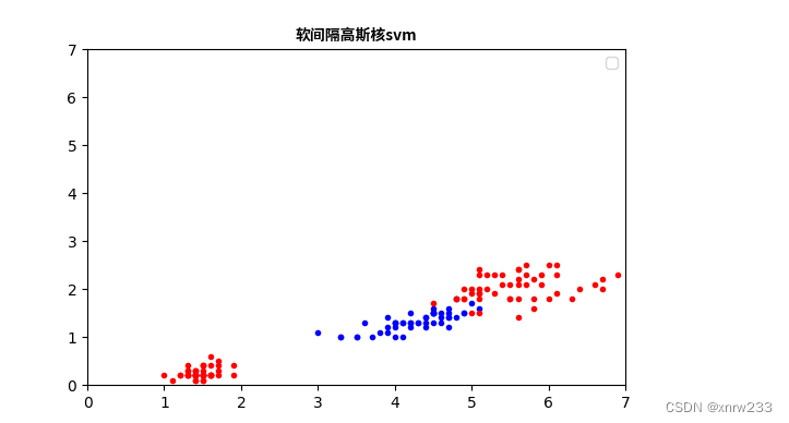
plt.title("软间隔高斯核svm",fontproperties=zhfont1)
plt.plot(X[:, 0][y==1], X[:, 1][y==1], "b.")
plt.plot(X[:, 0][y==-1], X[:, 1][y==-1], "r.")
plt.legend()
plt.axis([0, 7, 0, 7])

plt.figure(figsize=(14,4))
plt.subplot(121)
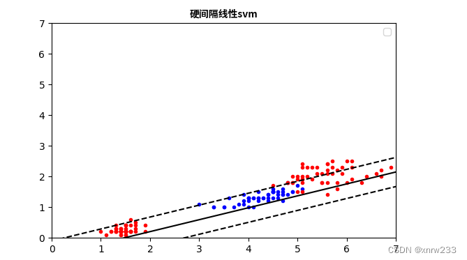
plt.title("硬间隔线性svm",fontproperties=zhfont1)
plt.plot(X[:, 0][y==1], X[:, 1][y==1], "b.")
plt.plot(X[:, 0][y==-1], X[:, 1][y==-1], "r.")
plot_svc_decision_boundary1(svm_clf2, 0, 7)
plt.legend()
plt.axis([0, 7, 0, 7])

plt.figure(figsize=(14,4))
plt.subplot(121)
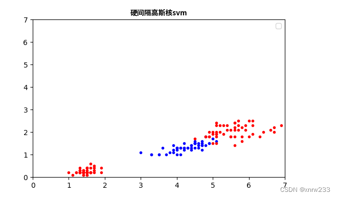
plt.title("硬间隔高斯核svm",fontproperties=zhfont1)
plt.plot(X[:, 0][y==1], X[:, 1][y==1], "b.")
plt.plot(X[:, 0][y==-1], X[:, 1][y==-1], "r.")
plt.legend()
plt.axis([0, 7, 0, 7])

plt.show()

结果是：