机器学习--支持向量机(sklearn)

最新推荐文章于 2024-03-13 22:15:57 发布

想成为风筝

最新推荐文章于 2024-03-13 22:15:57 发布

阅读量3.1k

点赞数 4

分类专栏：机器学习（sklearn）文章标签：机器学习支持向量机 sklearn

本文链接：https://blog.csdn.net/weixin_50918736/article/details/125747618

版权

机器学习（sklearn）专栏收录该内容

7 篇文章 0 订阅

订阅专栏

机器学习–支持向量机

1.1 线性可分支持向量机（硬间隔支持向量机）

训练数据集
$T={ (x_1,y_1),(x_2,y_2),…,(x_N,y_N)} $
当 $y_i=+1$ 时，称 $x_i$ 为正例；当 $y_i=-1$ 时，称 $x_i$ 为负例， $x_i,y_i)$ 称为样本点。
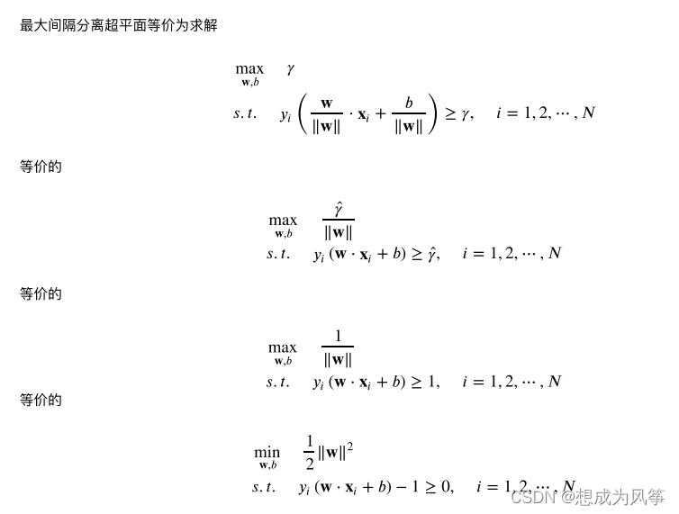
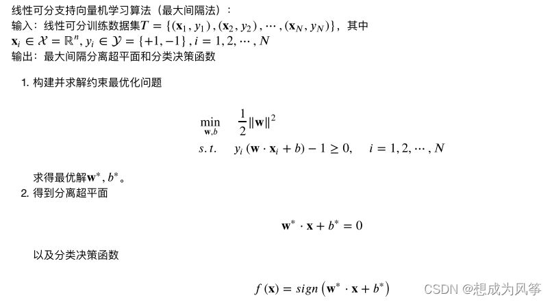
线性可分⽀持向量机（硬间隔⽀持向量机）：给定线性可分训练数据集，通过间隔最⼤化或等价地求解相应地凸⼆次规划问题学习得到分离超平⾯为
$w^* × x + b^* = 0$
以及相应的分类决策函数：
$f(x)=sign(s^* × x + b^*)$
称为线型可分支持向量机。其中 $w^*和b^*$ 为感知机模型参数。 $w^*$ 叫做权值， $b^*$ 叫作偏置。
超平面 $（ w, b ）$ 关于样本点 $x_i,y_i)$ 的函数间隔为：
$γ_i^* = y_i(w×x_i+b)$
超平面 $(w, b)$ 关于训练集 $T$ 的函数间隔：
$γ^*=min(γ_i ) ,i=1,2,..,N$
即超平面 $(w, b)$ 关于训练集 $T$ 中所有样本点 $x_i,y_i)$ 的函数间隔的最小值。
超平面 $(w, b)$ 关于样本点 $x_i,y_i)$ 的几何间隔为
$γ_i = y_i((w×x_i + b) /||w||)$
超平面 $(w, b)$ 关于训练集 $T$ 的几何间隔：
$γ=min(γ_i),i=1,2,...,N$
即超平面 $(w, b)$ 关于训练集 $T$ 中所有样本点 $x_i,y_i)$ 的几何间隔的最小值。
函数间隔和几何间隔的关系：
$γ_i = γ_i^* / ||w||$
$γ = γ^* / ||w||$
在这里插入图片描述

(硬间隔)支持向量:训练数据集的样本点中与分离超平面距离最近的样本点的实例，即使约束条件等号成立的样本点
$y_i(w×x_i + b)-1=0$
对 $y_i=+1$ 的正例点，支持向量在超平面
$H_1:w×x+b=1$
对 $y_i=-1$ 的正例点，支持向量在超平面
$H_2:w×x+b=-1$
$H_1,H_2$ 称为间隔边界。
$H_1和H_2之间的距离称为间隔,且|H_1H_2|=(1/||w||)+(1/||w||)=2/||w||)$
最优化问题的求解，使用拉格朗日法求解。

1.2线性支持向量机（软间隔支持向量机）

线性支持向量机（软间隔支持向量机）：给定线性不可分训练数据集，通过求解凸二次规划问题。
在这里插入图片描述
学习得到分离超平面为
$w^* × x + b^* = 0$
以及相应的分类决策函数
$f(x)=sign(w^* × x + b^*)$
称为线性支持向量机。

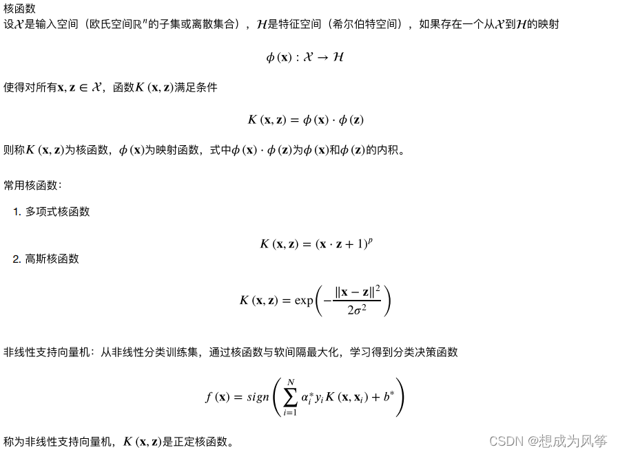
1.3非线性支持向量机（核技巧）

核函数
SVC的实现-sklearn库调用方式及参数解释
（1）LinearSVC实现了线性分类支持向量机

from sklearn.svm import LinearSVC
LinearSVC(penalty='l2',loss='squared_hinge',dual=True,tol=0.0001,C=1.0,multi_class='ovr', fit_intercept=True, intercept_scaling=1, class_weight=None,verbose=0,random_state=None, max_iter=1000)

参数：

C: 一个浮点数，罚项系数。C值越大对误分类的惩罚越大。
loss: 字符串，表示损失函数，可以为如下值：‘hinge’：此时为合页损失(标准的SVM损失函数)，‘squared_hinge’：合页损失函数的平方。
penalty: 字符串，指定‘l1’或者‘l2’，罚项范数。默认为‘l2’(他是标准的SVM范数)。
dual: 布尔值，如果为True，则解决对偶问题，如果是False，则解决原始问题。当n_samples>n_features是，倾向于采用False。
tol: 浮点数，指定终止迭代的阈值。
multi_class: 字符串，指定多分类的分类策略。‘ovr’：采用one-vs-rest策略。‘crammer_singer’: 多类联合分类，很少用，因为他计算量大，而且精度不会更佳，此时忽略loss,penalty,dual等参数。
fit_intecept: 布尔值，如果为True，则计算截距，即决策树中的常数项，否则忽略截距。
intercept_scaling: 浮点值，若提供了，则实例X变成向量[X,intercept_scaling]。此时相当于添加一个人工特征，该特征对所有实例都是常数值。
class_weight: 可以是个字典或者字符串‘balanced’。指定个各类的权重，若未提供，则认为类的权重为1。如果是字典，则指定每个类标签的权重。如果是‘balanced’，则每个累的权重是它出现频数的倒数。
verbose: 一个整数，表示是否开启verbose输出。
random_state: 一个整数或者一个RandomState实例，或者None。如果为整数，指定随机数生成器的种子。如果为RandomState，指定随机数生成器。
如果为None，指定使用默认的随机数生成器。
max_iter: 一个整数，指定最大迭代数。

属性：

coef_: 一个数组，它给出了各个特征的权重。
intercept_: 一个数组，它给出了截距。

方法

fit(X,y): 训练模型。
predict(X): 用模型进行预测，返回预测值。
score(X,y): 返回在(X,y)上的预测准确率。

（2）SVC实现了非线性分类支持向量机

from sklearn.svm import SVC
SVC(C=1.0, kernel='rbf', degree=3, gamma='auto_deprecated', coef0=0.0,shrinking=True,probability=False, tol=0.001, cache_size=200, class_weight=None,verbose=False,max_iter=-1, decision_function_shape='ovr', random_state=None)

参数：

C：惩罚参数，默认值是1.0C越大，相当于惩罚松弛变量，希望松弛变量接近0，即对误分类的惩罚增大，趋向于对训练集全分对的情况，这样对训练集测试时准确率很高，但泛化能力弱。C值小，对误分类的惩罚减小，允许容错，将他们当成噪声点，泛化能力较强。
kernel ：核函数，默认是rbf，可以是‘linear’, ‘poly’, ‘rbf’, ‘sigmoid’,
‘precomputed’(表示使用自定义的核函数矩阵)
degree ：多项式poly函数的阶数，默认是3，选择其他核函数时会被忽略。
gamma ： ‘rbf’,‘poly’ 和‘sigmoid’的核函数参数。默认是’auto’，则会选择1/n_features
coef0 ：核函数的常数项。对于‘poly’和 ‘sigmoid’有用。
probability ：是否采用概率估计.这必须在调用fit()之前启用，并且会f使it()方法速度变慢。默认为False
shrinking ：是否采用启发式收缩方式方法，默认为True
tol ：停止训练的误差值大小，默认为1e-3
cache_size ：指定训练所需要的内存，以MB为单位，默认为200MB。
class_weight ：类别的权重，字典形式传递。设置第几类的参数C为weight*C(SVC中的C)
verbose ：用于开启或者关闭迭代中间输出日志功能。
max_iter ：最大迭代次数。-1为无限制。
decision_function_shape ：‘ovo’, ‘ovr’ or None, default=‘ovr’
random_state ：数据洗牌时的种子值，int值

属性：

support_ : 支持向量的索引
support_vectors_ : 支持向量
n_support_ : 每个类别的支持向量的数目
dual_coef_ : 一个数组，形状为[n_class-1,n_SV]。对偶问题中，在分类决策函数中每一个支持向量的系数。
coef_ : 一个数组，形状为[n_class-1,n_features]。原始问题中，每个特征的系数。只有在linear kernel中有效。
intercept_ : 一个数组，形状为[n_class*(n_class-1)/2]。决策函数中的常数项。
fit_status_ : 整型，表示拟合的效果，如果正确拟合为0，否则为1
probA_ : array, shape = [n_class * (n_class-1) / 2]
probB_ : array, shape = [n_class * (n_class-1) / 2]

方法：

decision_function(X): 样本X到决策平面的距离
fit(X, y[, sample_weight]): 训练模型
get_params([deep]): 获取参数
predict(X): 预测
score(X, y[, sample_weight]): 返回预测的平均准确率
set_params(**params): 设定参数

（3）svm.LinearSVR

from sklearn.svm import LinearSVR
LinearSVR(epsilon=0.0, tol=0.0001, C=1.0, loss='epsilon_insensitive',fit_intercept=True,intercept_scaling=1.0, dual=True, verbose=0,random_state=None, max_iter=1000)

参数：

C: 一个浮点值，罚项系数。
loss:字符串，表示损失函数，可以为：
‘epsilon_insensitive’:此时损失函数为L_ϵ(标准的SVR)
‘squared_epsilon_insensitive’:此时损失函数为LϵLϵ
epsilon: 浮点数，用于lose中的ϵϵ参数。
dual: 布尔值。如果为True，则解决对偶问题，如果是False则解决原始问题。
tol: 浮点数，指定终止迭代的阈值。
fit_intercept: 布尔值。如果为True，则计算截距，否则忽略截距。
intercept_scaling: 浮点值。如果提供了，则实例X变成向量
[X,intercept_scaling]。此时相当于添加了一个人工特征，该特征对所有实例都是常数值。
verbose: 是否输出中间的迭代信息。
random_state: 指定随机数生成器的种子。
max_iter: 一个整数，指定最大迭代次数。

属性：

coef_: 一个数组，他给出了各个特征的权重。
intercept_: 一个数组，他给出了截距，及决策函数中的常数项。

方法：

fit(X,y): 训练模型。
predict(X): 用模型进行预测，返回预测值。
score(X,y): 返回性能得分。
（4）svm.SVR

from sklearn.svm import SVR
SVR(kernel='rbf', degree=3, gamma='auto', coef0=0.0, tol=0.001, C=1.0,epsilon=0.1, shrinking=True, cache_size=200, verbose=False, max_iter=-1)

参数：

C: 一个浮点值，罚项系数。
epsilon: 浮点数，用于lose中的ϵ参数。
kernel: 一个字符串，指定核函数。’linear’ : 线性核,‘poly’: 多项式核
‘rbf’: 默认值，高斯核函数,‘sigmoid’: Sigmoid核函数.‘precomputed’: 表示支持自定义核函数
degree: 一个整数，指定当核函数是多项式核函数时，多项式的系数。对于其它核函数该参数无效。
gamma: 一个浮点数。当核函数是’rbf’,’poly’,’sigmoid’时，核函数的系数。如果为‘auto’，则表示系数为1/n_features。
coef0: 浮点数，用于指定核函数中的自由项。只有当核函数是‘poly’和‘sigmoid’时有效。
shrinking: 布尔值。如果为True，则使用启发式收缩。
tol: 浮点数，指定终止迭代的阈值。
cache_size: 浮点值，指定了kernel cache的大小，单位为MB。
verbose: 指定是否开启verbose输出。
max_iter: 一个整数，指定最大迭代步数。

属性:

support_: 一个数组，形状为[n_SV]，支持向量的下标。
support_vectors_: 一个数组，形状为[n_SV,n_features]，支持向量。
n_support_: 一个数组，形状为[n_class]，每一个分类的支持向量个数。
dual_coef_: 一个数组，形状为[n_class-1,n_SV]。对偶问题中，在分类决策函数中每一个支持向量的系数。
coef_: 一个数组，形状为[n_class-1,n_features]。原始问题中，每个特征的系数。只有在linear kernel中有效。
intercept_: 一个数组，形状为[n_class*(n_class-1)/2]。决策函数中的常数项。

方法:

fit(X,y): 训练模型。
predict(X): 用模型进行预测，返回预测值。
score(X,y): 返回性能得分。

鸢尾花分类（支持向量机案例，直接调用sklearn）

import matplotlib.pyplot as plt
import numpy as np
from sklearn import datasets,linear_model,model_selection,svm

def load_data_classfication():
    iris = datasets.load_iris()
    x_train = iris.data
    y_train = iris.target
    return model_selection.train_test_split(x_train,y_train,test_size=0.2,random_state=0,stratify=y_train)

def test_SVC_linear(*data):
    x_train,x_test,y_train,y_test = data
    cls = svm.SVC(kernel='linear')
    cls.fit(x_train,y_train)
    print('Coefficients:%s.intercept %s'%(cls.coef_,cls.intercept_))
    print('Score:%.2f'%cls.score(x_test,y_test))
    
def test_SVC_poly(*data):
    x_train,x_test,y_train,y_test = data
    fig = plt.figure()
    
    degrees = range(1,20)
    train_scores = []
    test_scores = []
    for degree in degrees:
        cls = svm.SVC(kernel='poly',degree=degree)
        cls.fit(x_train,y_train)
        train_scores.append(cls.score(x_train,y_train))
        test_scores.append(cls.score(x_test,y_test))
    ax = fig.add_subplot(1,3,1)
    ax.plot(degrees,train_scores,label='Training score ',marker='+')
    ax.plot(degrees,test_scores,label='Testing score ',marker='o')
    ax.set_title('SVC_poly_degree')
    ax.set_xlabel('p')
    ax.set_ylabel('score')
    ax.set_ylim(0,1.05)
    ax.legend(loc='best',framealpha=0.5)
    
    gammas = range(1,20)
    train_scores = []
    test_scores = []
    for gamma in gammas:
        cls = svm.SVC(kernel='poly',gamma=gamma,degree=3)
        cls.fit(x_train,y_train)
        train_scores.append(cls.score(x_train,y_train))
        test_scores.append(cls.score(x_test,y_test))
    ax = fig.add_subplot(1,3,2)
    ax.plot(gammas,train_scores,label="Training score ",marker='+' )
    ax.plot(gammas,test_scores,label= " Testing score ",marker='o' )
    ax.set_title( "SVC_poly_gamma ")
    ax.set_xlabel(r"$\gamma$")
    ax.set_ylabel("score")
    ax.set_ylim(0,1.05)
    ax.legend(loc="best",framealpha=0.5)
    
    rs=range(0,20)
    train_scores=[]
    test_scores=[]
    for r in rs:
        cls=svm.SVC(kernel='poly',gamma=10,degree=3,coef0=r)
        cls.fit(X_train,y_train)
        train_scores.append(cls.score(X_train,y_train))
        test_scores.append(cls.score(X_test, y_test))
    ax=fig.add_subplot(1,3,3)
    ax.plot(rs,train_scores,label="Training score ",marker='+' )
    ax.plot(rs,test_scores,label= " Testing score ",marker='o' )
    ax.set_title( "SVC_poly_r ")
    ax.set_xlabel(r"r")
    ax.set_ylabel("score")
    ax.set_ylim(0,1.05)
    ax.legend(loc="best",framealpha=0.5)
    plt.show()
    
def test_SVC_rbf(*data):
    X_train,X_test,y_train,y_test=data
    gammas=range(1,20)
    train_scores=[]
    test_scores=[]
    for gamma in gammas:
        cls=svm.SVC(kernel='rbf',gamma=gamma)
        cls.fit(X_train,y_train)
        train_scores.append(cls.score(X_train,y_train))
        test_scores.append(cls.score(X_test, y_test))
    fig=plt.figure()
    ax=fig.add_subplot(1,1,1)
    ax.plot(gammas,train_scores,label="Training score ",marker='+' )
    ax.plot(gammas,test_scores,label= " Testing score ",marker='o' )
    ax.set_title( "SVC_rbf")
    ax.set_xlabel(r"$\gamma$")
    ax.set_ylabel("score")
    ax.set_ylim(0,1.05)
    ax.legend(loc="best",framealpha=0.5)
    plt.show()

def test_SVC_sigmoid(*data):
    X_train,X_test,y_train,y_test=data
    fig=plt.figure()
    gammas=np.logspace(-2,1)
    train_scores=[]
    test_scores=[]

    for gamma in gammas:
        cls=svm.SVC(kernel='sigmoid',gamma=gamma,coef0=0)
        cls.fit(X_train,y_train)
        train_scores.append(cls.score(X_train,y_train))
        test_scores.append(cls.score(X_test, y_test))
    ax=fig.add_subplot(1,2,1)
    ax.plot(gammas,train_scores,label="Training score ",marker='+' )
    ax.plot(gammas,test_scores,label= " Testing score ",marker='o' )
    ax.set_title( "SVC_sigmoid_gamma ")
    ax.set_xscale("log")
    ax.set_xlabel(r"$\gamma$")
    ax.set_ylabel("score")
    ax.set_ylim(0,1.05)
    ax.legend(loc="best",framealpha=0.5)
    
    rs=np.linspace(0,5)
    train_scores=[]
    test_scores=[]

    for r in rs:
        cls=svm.SVC(kernel='sigmoid',coef0=r,gamma=0.01)
        cls.fit(X_train,y_train)
        train_scores.append(cls.score(X_train,y_train))
        test_scores.append(cls.score(X_test, y_test))
    ax=fig.add_subplot(1,2,2)
    ax.plot(rs,train_scores,label="Training score ",marker='+' )
    ax.plot(rs,test_scores,label= " Testing score ",marker='o' )
    ax.set_title( "SVC_sigmoid_r ")
    ax.set_xlabel(r"r")
    ax.set_ylabel("score")
    ax.set_ylim(0,1.05)
    ax.legend(loc="best",framealpha=0.5)
    plt.show()
if __name__ == "__main__":
    X_train,X_test,y_train,y_test=load_data_classfication()
    test_SVC_linear(X_train,X_test,y_train,y_test)
    test_SVC_poly(X_train,X_test,y_train,y_test)
    test_SVC_rbf(X_train,X_test,y_train,y_test)
    test_SVC_sigmoid(X_train,X_test,y_train,y_test)