Canny边缘检测算法

最新推荐文章于 2024-04-18 10:18:54 发布

@kc++

最新推荐文章于 2024-04-18 10:18:54 发布

阅读量2.3k

点赞数 8

分类专栏： Computer Vision 文章标签：算法计算机视觉人工智能

本文链接：https://blog.csdn.net/m0_63260018/article/details/131160388

版权

Computer Vision 专栏收录该内容

14 篇文章 7 订阅

订阅专栏

Canny算法

Canny是目前最优秀的边缘检测算法之一，在传统机器学习算法当中，Canny是最优秀的算法，但是有深度学习的方法要比Canny好。Canny算法的目标是找到一个最优的边缘，其最优边缘的定义为：

好的检测：算法能够尽可能的标出图像中的实际边缘
好的定位：标识出的边缘要与实际图像中的边缘尽可能接近
最小响应：图像中的边缘只能标记一次

步骤

对图像进行灰度化
对图像进行高斯滤波：
根据待滤波的像素点及其邻域点的灰度值按照一定的参数规则进行加权平均。这样
可以有效滤去理想图像中叠加的高频噪声。
检测图像中的水平、垂直和对角边缘（如Prewitt，Sobel算子等）。
对梯度幅值进行非极大值抑制
用双阈值算法检测和连接边缘

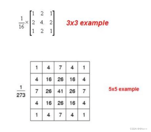
高斯平滑

高斯平滑水平和垂直方向呈现高斯分布，更突出了中心点在像素平滑后的权重，相比于均值滤波而言，有着更好的平滑效果。
在这里插入图片描述
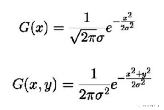
**重要的是需要理解，**高斯卷积核大小的选择将影响Canny检测器的性能：

尺寸越大，检测器对噪声的敏感度越低，但是边缘检测的定位误差也将略有增加。**一般5x5是一个比较不错的trade off。**这里解释一下为什么要寻找一个适中的trade off，因为实际上滤波和边缘检测是两个互相对立的东西，因为滤波是滤掉图像中的的高频成分达到降噪的目的，而边缘检测检测的也是高频成分，如果滤波太明显，在极端情况下，可能出现边缘消失的情况，所以我们需要一个适中的trade off，这个trade off来自于工程经验。

在这里插入图片描述

非极大值抑制

非极大值抑制，简称为NMS算法，英文为Non-Maximum Suppression。

其思想是搜素局部最大值，抑制非极大值。

NMS算法在不同应用中的具体实现不太一样，但思想是一样的。

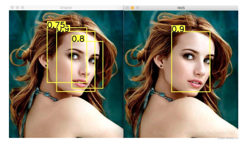
为什么要用非极大值抑制？

以目标检测为例：目标检测的过程中在同一目标的位置上会产生大量的候选框，这些候选框相互之间可能会有重叠，此时我们需要利用非极大值抑制找到最佳的目标边界框，消除冗余的边界框。

对于重叠的候选框，计算他们的重叠部分，若大于规定阈值，则删除；低于阈值则保留。对于无重叠的候选框，都保留。
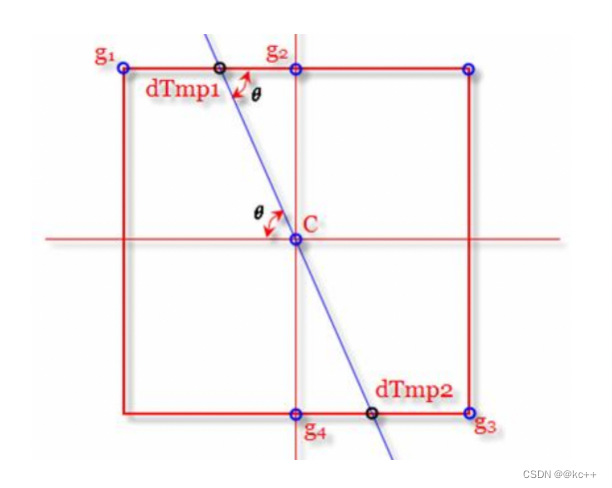
通俗意义上是指寻找像素点局部最大值，将非极大值点所对应的灰度值置为0，这样可以剔除掉一大部分非边缘的点。

将当前像素的梯度强度与沿正负梯度方向上的两个像素进行比较。
如果当前像素的梯度强度与另外两个像素相比最大，则该像素点保留为边缘点，否则该像素点将被抑制（灰度值置为0）。其中蓝色的线为梯度线，方向为C点的梯度方向，那么8领域中的最大值一定是在梯度线上

用双阈值算法检测（滞后阈值）
完成非极大值抑制后，会得到一个二值图像，非边缘的点灰度值均为0，可能为边缘的局部灰度极大值点可设置其灰度为128（或其他）。这样一个检测结果还是包含了很多由噪声及其他原因造成的假边缘。因此还需要进一步的处理。

双阈值检测：

如果边缘像素的梯度值高于高阈值，则将其标记为强边缘像素
如果边缘像素的梯度值小于高阈值并且大于低阈值，则将其标记为弱边缘像素
如果边缘像素的梯度值小于低阈值，则会被抑制
大于高阈值为强边缘，小于低阈值不是边缘。介于中间是弱边缘。
阈值的选择取决于给定输入图像的内容。

抑制孤立低阈值点

到目前为止，被划分为强边缘的像素点已经被确定为边缘，因为它们是从图像中的真实边缘中提取出来的。
然而，对于弱边缘像素，将会有一些争论，因为这些像素可以从真实边缘提取也可以是因噪声或颜色变化引起的。
为了获得准确的结果，应该抑制由后者引起的弱边缘：

通常，由真实边缘引起的弱边缘像素将连接到强边缘像素，而噪声响应未连接。
为了跟踪边缘连接，通过查看弱边缘像素及其8个邻域像素，只要其中一个为强边缘像素，则该弱边缘点就可以保留为真实的边缘。

代码实现

手动实现

在这里插入代码片import numpy as np
import matplotlib.pyplot as plt
import math
 
if __name__ == '__main__':
    pic_path = 'lenna.png' 
    img = plt.imread(pic_path)
    if pic_path[-4:] == '.png':  # .png图片在这里的存储格式是0到1的浮点数，所以要扩展到255再计算
        img = img * 255  # 还是浮点数类型
    img = img.mean(axis=-1)  # 取均值就是灰度化了
 
    # 1、高斯平滑
    #sigma = 1.52  # 高斯平滑时的高斯核参数，标准差，可调
    sigma = 0.5  # 高斯平滑时的高斯核参数，标准差，可调
    dim = int(np.round(6 * sigma + 1))  # round是四舍五入函数，根据标准差求高斯核是几乘几的，也就是维度
    if dim % 2 == 0:  # 最好是奇数,不是的话加一
        dim += 1
    Gaussian_filter = np.zeros([dim, dim])  # 存储高斯核，这是数组不是列表了
    tmp = [i-dim//2 for i in range(dim)]  # 生成一个序列
    n1 = 1/(2*math.pi*sigma**2)  # 计算高斯核
    n2 = -1/(2*sigma**2)
    for i in range(dim):
        for j in range(dim):
            Gaussian_filter[i, j] = n1*math.exp(n2*(tmp[i]**2+tmp[j]**2))
    Gaussian_filter = Gaussian_filter / Gaussian_filter.sum()
    dx, dy = img.shape
    img_new = np.zeros(img.shape)  # 存储平滑之后的图像，zeros函数得到的是浮点型数据
    tmp = dim//2
    img_pad = np.pad(img, ((tmp, tmp), (tmp, tmp)), 'constant')  # 边缘填补
    for i in range(dx):
        for j in range(dy):
            img_new[i, j] = np.sum(img_pad[i:i+dim, j:j+dim]*Gaussian_filter)
    plt.figure(1)
    plt.imshow(img_new.astype(np.uint8), cmap='gray')  # 此时的img_new是255的浮点型数据，强制类型转换才可以，gray灰阶
    plt.axis('off')
 
    # 2、求梯度。以下两个是滤波求梯度用的sobel矩阵（检测图像中的水平、垂直和对角边缘）
    sobel_kernel_x = np.array([[-1, 0, 1], [-2, 0, 2], [-1, 0, 1]])
    sobel_kernel_y = np.array([[1, 2, 1], [0, 0, 0], [-1, -2, -1]])
    img_tidu_x = np.zeros(img_new.shape)  # 存储梯度图像
    img_tidu_y = np.zeros([dx, dy])
    img_tidu = np.zeros(img_new.shape)
    img_pad = np.pad(img_new, ((1, 1), (1, 1)), 'constant')  # 边缘填补，根据上面矩阵结构所以写1
    for i in range(dx):
        for j in range(dy):
            img_tidu_x[i, j] = np.sum(img_pad[i:i+3, j:j+3]*sobel_kernel_x)  # x方向
            img_tidu_y[i, j] = np.sum(img_pad[i:i+3, j:j+3]*sobel_kernel_y)  # y方向
            img_tidu[i, j] = np.sqrt(img_tidu_x[i, j]**2 + img_tidu_y[i, j]**2)
    img_tidu_x[img_tidu_x == 0] = 0.00000001
    angle = img_tidu_y/img_tidu_x
    plt.figure(2)
    plt.imshow(img_tidu.astype(np.uint8), cmap='gray')
    plt.axis('off')
 
    # 3、非极大值抑制
    img_yizhi = np.zeros(img_tidu.shape)
    for i in range(1, dx-1):
        for j in range(1, dy-1):
            flag = True  # 在8邻域内是否要抹去做个标记
            temp = img_tidu[i-1:i+2, j-1:j+2]  # 梯度幅值的8邻域矩阵
            if angle[i, j] <= -1:  # 使用线性插值法判断抑制与否
                num_1 = (temp[0, 1] - temp[0, 0]) / angle[i, j] + temp[0, 1]
                num_2 = (temp[2, 1] - temp[2, 2]) / angle[i, j] + temp[2, 1]
                if not (img_tidu[i, j] > num_1 and img_tidu[i, j] > num_2):
                    flag = False
            elif angle[i, j] >= 1:
                num_1 = (temp[0, 2] - temp[0, 1]) / angle[i, j] + temp[0, 1]
                num_2 = (temp[2, 0] - temp[2, 1]) / angle[i, j] + temp[2, 1]
                if not (img_tidu[i, j] > num_1 and img_tidu[i, j] > num_2):
                    flag = False
            elif angle[i, j] > 0:
                num_1 = (temp[0, 2] - temp[1, 2]) * angle[i, j] + temp[1, 2]
                num_2 = (temp[2, 0] - temp[1, 0]) * angle[i, j] + temp[1, 0]
                if not (img_tidu[i, j] > num_1 and img_tidu[i, j] > num_2):
                    flag = False
            elif angle[i, j] < 0:
                num_1 = (temp[1, 0] - temp[0, 0]) * angle[i, j] + temp[1, 0]
                num_2 = (temp[1, 2] - temp[2, 2]) * angle[i, j] + temp[1, 2]
                if not (img_tidu[i, j] > num_1 and img_tidu[i, j] > num_2):
                    flag = False
            if flag:
                img_yizhi[i, j] = img_tidu[i, j]
    plt.figure(3)
    plt.imshow(img_yizhi.astype(np.uint8), cmap='gray')
    plt.axis('off')
 
    # 4、双阈值检测，连接边缘。遍历所有一定是边的点,查看8邻域是否存在有可能是边的点，进栈
    lower_boundary = img_tidu.mean() * 0.5
    high_boundary = lower_boundary * 3  # 这里我设置高阈值是低阈值的三倍
    zhan = []
    for i in range(1, img_yizhi.shape[0]-1):  # 外圈不考虑了
        for j in range(1, img_yizhi.shape[1]-1):
            if img_yizhi[i, j] >= high_boundary:  # 取，一定是边的点
                img_yizhi[i, j] = 255
                zhan.append([i, j])
            elif img_yizhi[i, j] <= lower_boundary:  # 舍
                img_yizhi[i, j] = 0
 
    while not len(zhan) == 0:
        temp_1, temp_2 = zhan.pop()  # 出栈
        a = img_yizhi[temp_1-1:temp_1+2, temp_2-1:temp_2+2]
        if (a[0, 0] < high_boundary) and (a[0, 0] > lower_boundary):
            img_yizhi[temp_1-1, temp_2-1] = 255  # 这个像素点标记为边缘
            zhan.append([temp_1-1, temp_2-1])  # 进栈
        if (a[0, 1] < high_boundary) and (a[0, 1] > lower_boundary):
            img_yizhi[temp_1 - 1, temp_2] = 255
            zhan.append([temp_1 - 1, temp_2])
        if (a[0, 2] < high_boundary) and (a[0, 2] > lower_boundary):
            img_yizhi[temp_1 - 1, temp_2 + 1] = 255
            zhan.append([temp_1 - 1, temp_2 + 1])
        if (a[1, 0] < high_boundary) and (a[1, 0] > lower_boundary):
            img_yizhi[temp_1, temp_2 - 1] = 255
            zhan.append([temp_1, temp_2 - 1])
        if (a[1, 2] < high_boundary) and (a[1, 2] > lower_boundary):
            img_yizhi[temp_1, temp_2 + 1] = 255
            zhan.append([temp_1, temp_2 + 1])
        if (a[2, 0] < high_boundary) and (a[2, 0] > lower_boundary):
            img_yizhi[temp_1 + 1, temp_2 - 1] = 255
            zhan.append([temp_1 + 1, temp_2 - 1])
        if (a[2, 1] < high_boundary) and (a[2, 1] > lower_boundary):
            img_yizhi[temp_1 + 1, temp_2] = 255
            zhan.append([temp_1 + 1, temp_2])
        if (a[2, 2] < high_boundary) and (a[2, 2] > lower_boundary):
            img_yizhi[temp_1 + 1, temp_2 + 1] = 255
            zhan.append([temp_1 + 1, temp_2 + 1])
 
    for i in range(img_yizhi.shape[0]):
        for j in range(img_yizhi.shape[1]):
            if img_yizhi[i, j] != 0 and img_yizhi[i, j] != 255:
                img_yizhi[i, j] = 0
 
    # 绘图
    plt.figure(4)
    plt.imshow(img_yizhi.astype(np.uint8), cmap='gray')
    plt.axis('off')  # 关闭坐标刻度值
    plt.show()

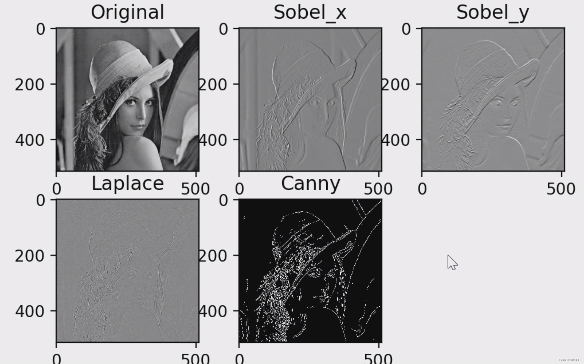
Sobel_laplace_Canny三种算法的比较

#!/usr/bin/env python
# encoding=gbk

import cv2  
import numpy as np  
from matplotlib import pyplot as plt  

img = cv2.imread("lenna.png",1)  

img_gray = cv2.cvtColor(img, cv2.COLOR_RGB2GRAY)  

'''
Sobel算子
Sobel算子函数原型如下：
dst = cv2.Sobel(src, ddepth, dx, dy[, dst[, ksize[, scale[, delta[, borderType]]]]]) 
前四个是必须的参数：
第一个参数是需要处理的图像；
第二个参数是图像的深度，-1表示采用的是与原图像相同的深度。目标图像的深度必须大于等于原图像的深度；
dx和dy表示的是求导的阶数，0表示这个方向上没有求导，一般为0、1、2。
其后是可选的参数：
dst是目标图像；
ksize是Sobel算子的大小，必须为1、3、5、7。
scale是缩放导数的比例常数，默认情况下没有伸缩系数；
delta是一个可选的增量，将会加到最终的dst中，同样，默认情况下没有额外的值加到dst中；
borderType是判断图像边界的模式。这个参数默认值为cv2.BORDER_DEFAULT。
'''

img_sobel_x = cv2.Sobel(img_gray, cv2.CV_64F, 1, 0, ksize=3)  # 对x求导
img_sobel_y = cv2.Sobel(img_gray, cv2.CV_64F, 0, 1, ksize=3)  # 对y求导

# Laplace 算子  
img_laplace = cv2.Laplacian(img_gray, cv2.CV_64F, ksize=3)  

# Canny 算子  
img_canny = cv2.Canny(img_gray, 100 , 150)  

plt.subplot(231), plt.imshow(img_gray, "gray"), plt.title("Original")  
plt.subplot(232), plt.imshow(img_sobel_x, "gray"), plt.title("Sobel_x")  
plt.subplot(233), plt.imshow(img_sobel_y, "gray"), plt.title("Sobel_y")  
plt.subplot(234), plt.imshow(img_laplace,  "gray"), plt.title("Laplace")  
plt.subplot(235), plt.imshow(img_canny, "gray"), plt.title("Canny")  
plt.show()

在这里插入图片描述

调用接口

#!/usr/bin/env python
# encoding=gbk

import cv2
import numpy as np

'''
cv2.Canny(image, threshold1, threshold2[, edges[, apertureSize[, L2gradient ]]])   
必要参数：
第一个参数是需要处理的原图像，该图像必须为单通道的灰度图；
第二个参数是滞后阈值1；
第三个参数是滞后阈值2。
'''

img = cv2.imread("lenna.png", 1)
gray = cv2.cvtColor(img, cv2.COLOR_BGR2GRAY)
cv2.imshow("canny", cv2.Canny(gray, 200, 300))
cv2.waitKey()
cv2.destroyAllWindows()

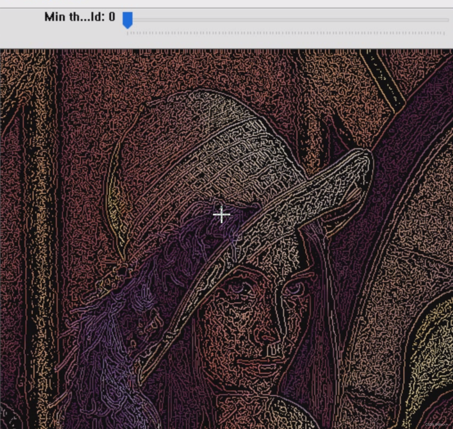
程序优化，增加调节杆，查看阈值对结果的影响

#!/usr/bin/env python
# encoding=gbk
 
'''
Canny边缘检测：优化的程序
'''
import cv2
import numpy as np 
 
def CannyThreshold(lowThreshold):  
    detected_edges = cv2.GaussianBlur(gray,(3,3),0) #高斯滤波 
    detected_edges = cv2.Canny(detected_edges,
            lowThreshold,
            lowThreshold*ratio,
            apertureSize = kernel_size)  #边缘检测
 
     # just add some colours to edges from original image.  
    dst = cv2.bitwise_and(img,img,mask = detected_edges)  #用原始颜色添加到检测的边缘上
    cv2.imshow('canny demo',dst)  
  
 
lowThreshold = 0  
max_lowThreshold = 100  
ratio = 3  
kernel_size = 3  
  
img = cv2.imread('lenna.png')  
gray = cv2.cvtColor(img,cv2.COLOR_BGR2GRAY)  #转换彩色图像为灰度图
  
cv2.namedWindow('canny demo')  
  
#设置调节杠,
'''
下面是第二个函数，cv2.createTrackbar()
共有5个参数，其实这五个参数看变量名就大概能知道是什么意思了
第一个参数，是这个trackbar对象的名字
第二个参数，是这个trackbar对象所在面板的名字
第三个参数，是这个trackbar的默认值,也是调节的对象
第四个参数，是这个trackbar上调节的范围(0~count)
第五个参数，是调节trackbar时调用的回调函数名
'''
cv2.createTrackbar('Min threshold','canny demo',lowThreshold, max_lowThreshold, CannyThreshold)  
  
CannyThreshold(0)  # initialization  
if cv2.waitKey(0) == 27:  #wait for ESC key to exit cv2
    cv2.destroyAllWindows()

在这里插入图片描述

@kc++

关注

8
点赞
踩
16

收藏

觉得还不错? 一键收藏
1
评论
Canny边缘检测算法

Canny是目前最优秀的边缘检测算法之一，在传统机器学习算法当中，Canny是最优秀的算法，但是有深度学习的方法要比Canny好。高斯平滑水平和垂直方向呈现高斯分布，更突出了中心点在像素平滑后的权重，相比于均值滤波而言，有着更好的平滑效果。**重要的是需要理解，**高斯卷积核大小的选择将影响Canny检测器的性能：尺寸越大，检测器对噪声的敏感度越低，但是边缘检测的定位误差也将略有增加。**一般5x5是一个比较不错的trade off。
复制链接

扫一扫