实验四 图像增强

1.直方图计算

先来介绍以下什么叫做bin值

在这样一个8x8的数据中，像素范围为0-14的15个等级，先统计各个像素值的出现次数，出现的次数就是bin值

将bins划分为16个等级一共有看16位

常见的直方图属性：

dims：表示维度，对灰度图像来说只有一个通道
bins：表示维度中子区域大小划分，bins=256，划分为256个级别
range：表示值的范围，灰度值范围在【0-255】之间（转换到HSV空间时，H【0-300】S【0-180】）

直方图计算测试：

numpy返回的是每个bin的两端的范围值，⽽skimage返回的是每个bin的中间值

import matplotlib as plt
import numpy as np
from skimage import io, data, exposure

img = io.imread('OIP.jpg')

hist1 = np.histogram(img, bins=2)
hist2 = exposure.histogram(img, nbins = 2)
print(hist1)
print(hist2)

hist1

hist2

2.直方图绘制

arr: 需要计算直⽅图的⼀维数组

bins: 直⽅图的柱数，可选项，默认为10

normed: 是否将得到的直⽅图向量归⼀化。默认为0

facecolor: 直⽅图颜⾊

edgecolor: 直⽅图边框颜⾊

alpha: 透明度

histtype: 直⽅图类型，‘bar', ‘barstacked', ‘step', ‘stepfilled'

n, bins, patches = plt.hist(arr, bins=10, normed=0, facecolor='black', edgecolor='black',alpha=1，histtype='bar')

import matplotlib.pyplot as plt
from skimage import io

img = io.imread('OIP.jpg')
plt.figure('hist', figsize=(10, 5))
arr = img.flatten()
plt.subplot(121)
plt.imshow(img, cmap='gray')

plt.subplot(122)
n, bins, patches = plt.hist(arr, bins=256, facecolor='green', alpha=0.75, histtype='stepfilled',edgecolor='green')
plt.tight_layout()
plt.show()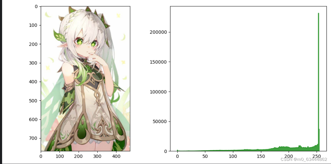

彩色三通道直方图：

import matplotlib.pyplot as plt
from skimage import io

img = io.imread('OIP.jpg')
plt.figure('hist', figsize=(10, 5))
arr = img.flatten()
plt.subplot(121)
plt.imshow(img, cmap='gray')
ar = img[:,:,0].flatten()
plt.subplot(122)
plt.hist(arr, bins=256, facecolor='red',edgecolor='red', alpha=0.75)
ag = img[:,:,1].flatten()
plt.hist(ag, bins=256, facecolor='green',edgecolor='green', alpha=0.75)
ab = img[:,:,2].flatten()
plt.hist(ab, bins=256, facecolor='blue',edgecolor='blue', alpha=0.75)

plt.tight_layout()
plt.show()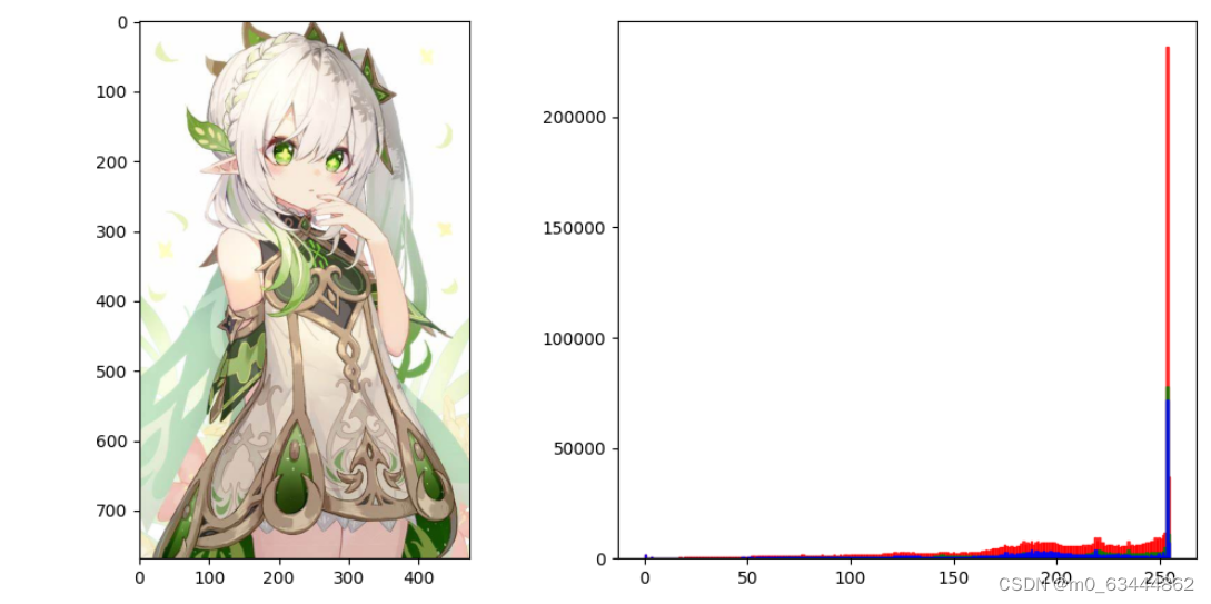

3.直方图均衡化

from skimage import exposure,io
import matplotlib.pyplot as plt

img=io.imread('OIP.jpg')
plt.figure("hist",figsize=(8,8))
arr=img.flatten()
plt.subplot(221)
plt.imshow(img, cmap='gray') #原始图像
plt.subplot(222)
plt.hist(arr, bins=256,edgecolor='None',facecolor='red')

img1=exposure.equalize_hist(img)
arr1=img1.flatten()
plt.subplot(223)
plt.imshow(img1,cmap = 'gray') #均衡化图像
plt.subplot(224)
plt.hist(arr1, bins=256,edgecolor='None',facecolor='red')
plt.show()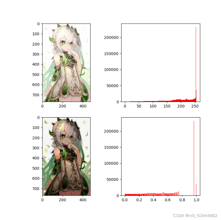

图像增强：

from PIL import Image
from PIL import ImageEnhance
from skimage import data
#原始图像
image=Image.open('OIP.jpg')
image.show()
#亮度增强
enh_bri = ImageEnhance.Brightness(image)
brightness = 1.5
image_brightened = enh_bri.enhance(brightness)
image_brightened.show()
#⾊度增强
enh_col = ImageEnhance.Color(image)
color = 1.5
image_colored = enh_col.enhance(color)
image_colored.show()
#对⽐度增强
enh_con = ImageEnhance.Contrast(image)
contrast = 1.5
image_contrasted = enh_con.enhance(contrast)
image_contrasted.show()
#锐度增强
enh_sha = ImageEnhance.Sharpness(image)
sharpness = 3.0
image_sharped = enh_sha.enhance(sharpness)
image_sharped.show()

直方图均衡化实质上是减少图像的灰度级来加大对比度，图像经均衡化处理之后，图像变得清晰，直方图中每个像素点的灰度级减少，但分布更加均匀，对比度更高。

（1）将原始函数的累积分布函数作为变换函数，只能产生近似均匀的直方图。

（2）在某些情况下，并不一定需要具有均匀直方图的图像。

滤波：

from PIL import ImageFilter
from PIL import Image
imgF = Image.open('OIP.jpg')
blurF = imgF.filter(ImageFilter.BLUR)
outF = imgF.filter(ImageFilter.DETAIL)
conF = imgF.filter(ImageFilter.CONTOUR)
edgeF = imgF.filter(ImageFilter.FIND_EDGES)
edge_enhF = imgF.filter(ImageFilter.EDGE_ENHANCE)
imgF.show()
blurF.show()
outF.show()
conF.show()
edgeF.show()
edge_enhF.show()

更改对比度：

from PIL import Image


def change_contrast(img, level):
    factor = (259 * (level + 255)) / (255 * (259 - level))

    def contrast(c):
        return 128 + factor * (c - 128)

    return img.point(contrast)


def change_contrast_multi(img, steps):
    width, height = img.size
    canvas = Image.new('RGB', (width * len(steps), height))
    for n, level in enumerate(steps):
        print(level)
        img_filtered = change_contrast(img, level)
        canvas.paste(img_filtered, (width * n, 0))
    return canvas


image = Image.open('OIP.jpg')
contrast_levels = [-50, -25, 0, 25, 50]
result = change_contrast_multi(image, contrast_levels)
result.save('output.jpg')

复盘：主要是直方图均衡化的原理要注意是概率密度函数的灰度级减少来增加对比度