


 本文通过具体实例,详细介绍了BP算法的过程推导、数值计算及代码实现。对比了使用numpy与PyTorch的不同效果,并探讨了激活函数、损失函数、步长等参数对训练结果的影响。
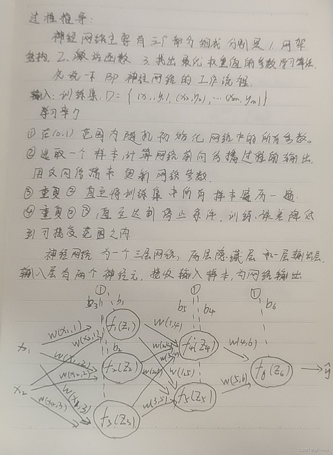
- 过程推导 - 了解BP原理
- 数值计算 - 手动计算,掌握细节
- 代码实现 - numpy手推 + pytorch自动
代码实现的要求:
- 对比【numpy】和【pytorch】程序,总结并陈述。
- 激活函数Sigmoid用PyTorch自带函数torch.sigmoid(),观察、总结并陈述。
- 激活函数Sigmoid改变为Relu,观察、总结并陈述。
- 损失函数MSE用PyTorch自带函数 t.nn.MSELoss()替代,观察、总结并陈述。
- 损失函数MSE改变为交叉熵,观察、总结并陈述。
- 改变步长,训练次数,观察、总结并陈述。
- 权值w1-w8初始值换为随机数,对比“指定权值”的结果,观察、总结并陈述。
- 权值w1-w8初始值换为0,观察、总结并陈述。
- 全面总结反向传播原理和编码实现,认真写心得体会。
目录
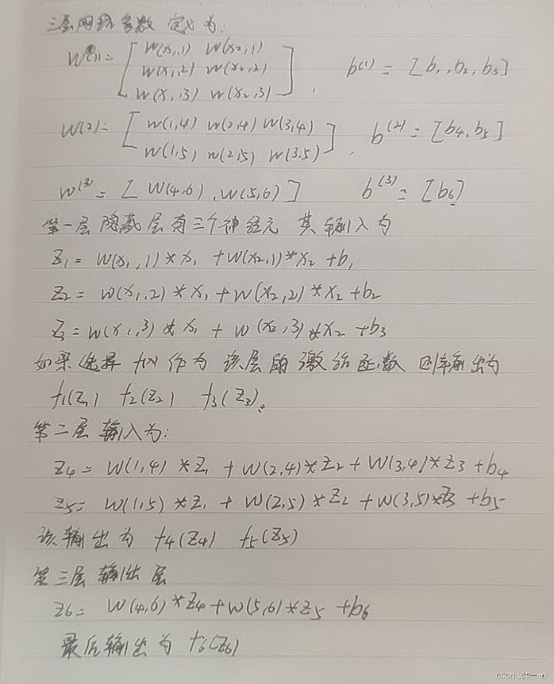
1. 过程推导
2. 数值计算
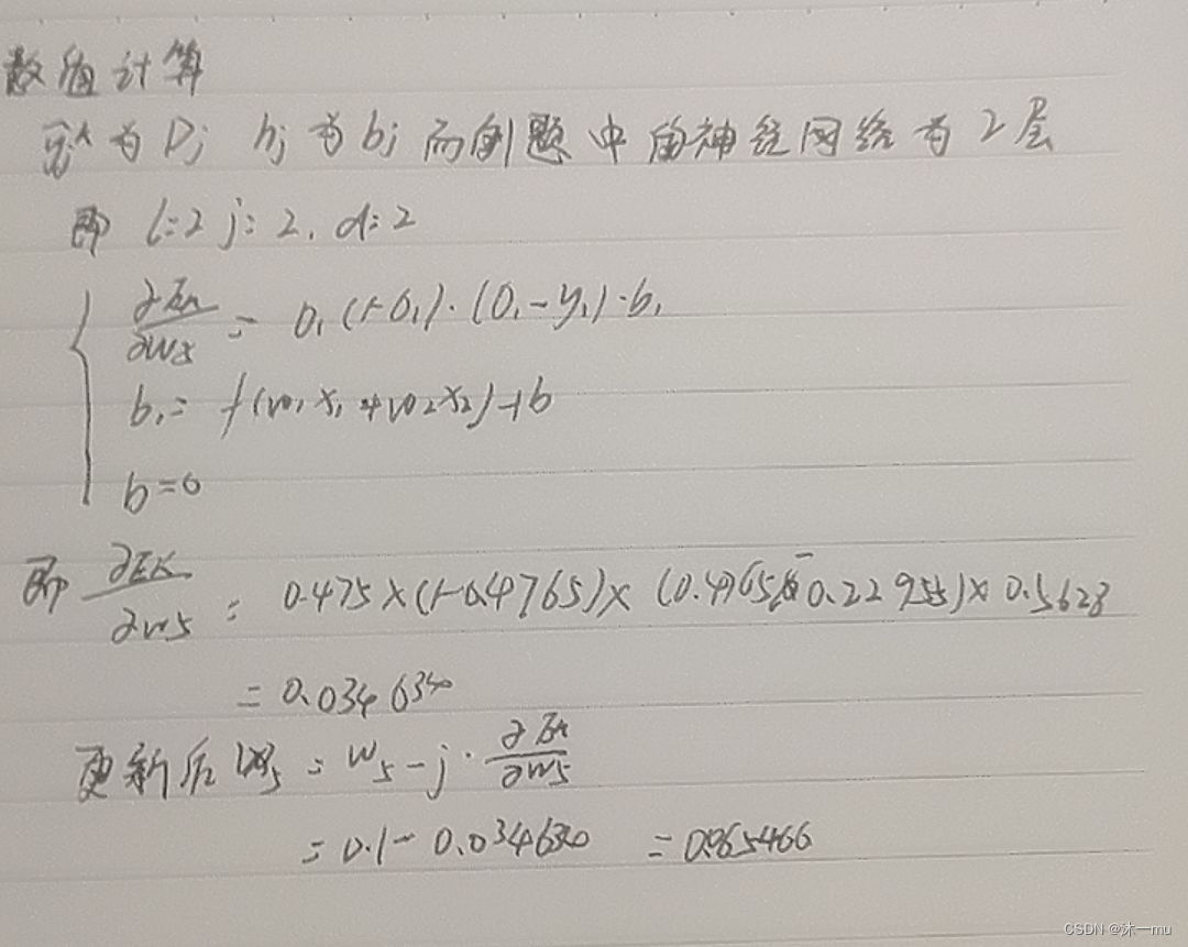
计算偏导数


3. 代码实现
3.1 numpy:
import numpy as np
def sigmoid(z):
a = 1 / (1 + np.exp(-z))
return a
def forward_propagate(x1, x2, y1, y2, w1, w2, w3, w4, w5, w6, w7, w8):
in_h1 = w1 * x1 + w3 * x2
out_h1 = sigmoid(in_h1)
in_h2 = w2 * x1 + w4 * x2
out_h2 = sigmoid(in_h2)
in_o1 = w5 * out_h1 + w7 * out_h2
out_o1 = sigmoid(in_o1)
in_o2 = w6 * out_h1 + w8 * out_h2
out_o2 = sigmoid(in_o2)
print("正向计算:o1 ,o2")
print(round(out_o1, 5), round(out_o2, 5))
error = (1 / 2) * (out_o1 - y1) ** 2 + (1 / 2) * (out_o2 - y2) ** 2
print("损失函数:均方误差")
print(round(error, 5))
return out_o1, out_o2, out_h1, out_h2
def back_propagate(out_o1, out_o2, out_h1, out_h2):
# 反向传播
d_o1 = out_o1 - y1
d_o2 = out_o2 - y2
# print(round(d_o1, 2), round(d_o2, 2))
d_w5 = d_o1 * out_o1 * (1 - out_o1) * out_h1
d_w7 = d_o1 * out_o1 * (1 - out_o1) * out_h2
# print(round(d_w5, 2), round(d_w7, 2))
d_w6 = d_o2 * out_o2 * (1 - out_o2) * out_h1
d_w8 = d_o2 * out_o2 * (1 - out_o2) * out_h2
# print(round(d_w6, 2), round(d_w8, 2))
d_w1 = (d_w5 + d_w6) * out_h1 * (1 - out_h1) * x1
d_w3 = (d_w5 + d_w6) * out_h1 * (1 - out_h1) * x2
# print(round(d_w1, 2), round(d_w3, 2))
d_w2 = (d_w7 + d_w8) * out_h2 * (1 - out_h2) * x1
d_w4 = (d_w7 + d_w8) * out_h2 * (1 - out_h2) * x2
# print(round(d_w2, 2), round(d_w4, 2))
print("反向传播:误差传给每个权值")
print(round(d_w1, 5), round(d_w2, 5), round(d_w3, 5), round(d_w4, 5), round(d_w5, 5), round(d_w6, 5),
round(d_w7, 5), round(d_w8, 5))
return d_w1, d_w2, d_w3, d_w4, d_w5, d_w6, d_w7, d_w8
def update_w(w1, w2, w3, w4, w5, w6, w7, w8):
# 步长
step = 5
w1 = w1 - step * d_w1
w2 = w2 - step * d_w2
w3 = w3 - step * d_w3
w4 = w4 - step * d_w4
w5 = w5 - step * d_w5
w6 = w6 - step * d_w6
w7 = w7 - step * d_w7
w8 = w8 - step * d_w8
return w1, w2, w3, w4, w5, w6, w7, w8
if __name__ == "__main__":
w1, w2, w3, w4, w5, w6, w7, w8 = 0.2, -0.4, 0.5, 0.6, 0.1, -0.5, -0.3, 0.8
x1, x2 = 0.5, 0.3
y1, y2 = 0.23, -0.07
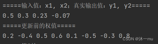
print("=====输入值:x1, x2;真实输出值:y1, y2=====")
print(x1, x2, y1, y2)
print("=====更新前的权值=====")
print(round(w1, 2), round(w2, 2), round(w3, 2), round(w4, 2), round(w5, 2), round(w6, 2), round(w7, 2),
round(w8, 2))
for i in range(1000):
print("=====第" + str(i) + "轮=====")
out_o1, out_o2, out_h1, out_h2 = forward_propagate(x1, x2, y1, y2, w1, w2, w3, w4, w5, w6, w7, w8)
d_w1, d_w2, d_w3, d_w4, d_w5, d_w6, d_w7, d_w8 = back_propagate(out_o1, out_o2, out_h1, out_h2)
w1, w2, w3, w4, w5, w6, w7, w8 = update_w(w1, w2, w3, w4, w5, w6, w7, w8)
print("更新后的权值")
print(round(w1, 2), round(w2, 2), round(w3, 2), round(w4, 2), round(w5, 2), round(w6, 2), round(w7, 2),
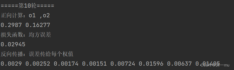
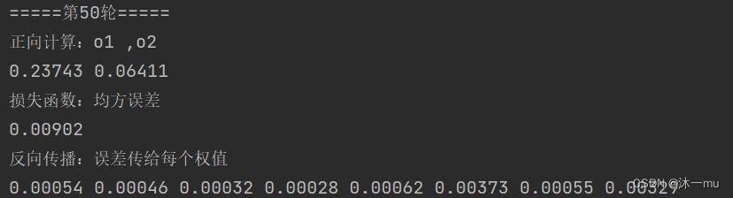
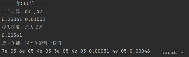
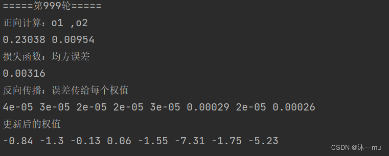
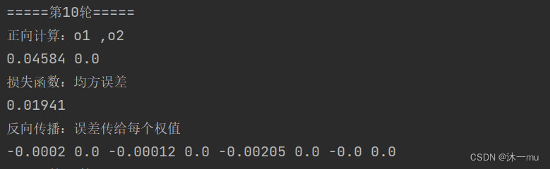
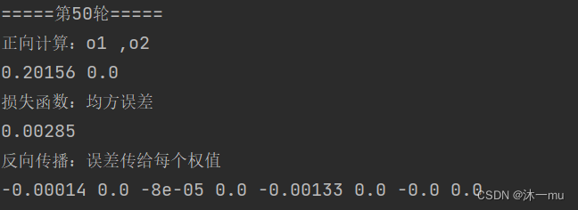
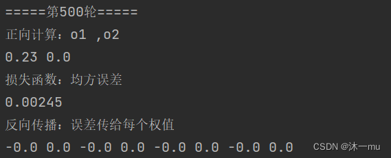
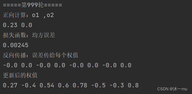
round(w8, 2))执行结果:
3.2 pytorch:
import torch

x1, x2 = torch.Tensor([0.5]), torch.Tensor([0.3])
y1, y2 = torch.Tensor([0.23]), torch.Tensor([-0.07])
print("=====输入值:x1, x2;真实输出值:y1, y2=====")
print(x1, x2, y1, y2)
w1, w2, w3, w4, w5, w6, w7, w8 = torch.Tensor([0.2]), torch.Tensor([-0.4]), torch.Tensor([0.5]), torch.Tensor(
    [0.6]), torch.Tensor([0.1]), torch.Tensor([-0.5]), torch.Tensor([-0.3]), torch.Tensor([0.8])  # 权重初始值
w1.requires_grad = True
w2.requires_grad = True
w3.requires_grad = True
w4.requires_grad = True
w5.requires_grad = True
w6.requires_grad = True
w7.requires_grad = True
w8.requires_grad = True


def sigmoid(z):
    a = 1 / (1 + torch.exp(-z))
    return a


def forward_propagate(x1, x2):
    in_h1 = w1 * x1 + w3 * x2
    out_h1 = sigmoid(in_h1)  # out_h1 = torch.sigmoid(in_h1)
    in_h2 = w2 * x1 + w4 * x2
    out_h2 = sigmoid(in_h2)  # out_h2 = torch.sigmoid(in_h2)

    in_o1 = w5 * out_h1 + w7 * out_h2
    out_o1 = sigmoid(in_o1)  # out_o1 = torch.sigmoid(in_o1)
    in_o2 = w6 * out_h1 + w8 * out_h2
    out_o2 = sigmoid(in_o2)  # out_o2 = torch.sigmoid(in_o2)

    print("正向计算:o1 ,o2")
    print(out_o1.data, out_o2.data)

    return out_o1, out_o2


def loss_fuction(x1, x2, y1, y2):  # 损失函数
    y1_pred, y2_pred = forward_propagate(x1, x2)  # 前向传播
    loss = (1 / 2) * (y1_pred - y1) ** 2 + (1 / 2) * (y2_pred - y2) ** 2  # 考虑 : t.nn.MSELoss()
    print("损失函数(均方误差):", loss.item())
    return loss


def update_w(w1, w2, w3, w4, w5, w6, w7, w8):
    # 步长
    step = 1
    w1.data = w1.data - step * w1.grad.data
    w2.data = w2.data - step * w2.grad.data
    w3.data = w3.data - step * w3.grad.data
    w4.data = w4.data - step * w4.grad.data
    w5.data = w5.data - step * w5.grad.data
    w6.data = w6.data - step * w6.grad.data
    w7.data = w7.data - step * w7.grad.data
    w8.data = w8.data - step * w8.grad.data
    w1.grad.data.zero_()  # 注意:将w中所有梯度清零
    w2.grad.data.zero_()
    w3.grad.data.zero_()
    w4.grad.data.zero_()
    w5.grad.data.zero_()
    w6.grad.data.zero_()
    w7.grad.data.zero_()
    w8.grad.data.zero_()
    return w1, w2, w3, w4, w5, w6, w7, w8


if __name__ == "__main__":

    print("=====更新前的权值=====")
    print(w1.data, w2.data, w3.data, w4.data, w5.data, w6.data, w7.data, w8.data)

    for i in range(1):
        print("=====第" + str(i) + "轮=====")
        L = loss_fuction(x1, x2, y1, y2)  # 前向传播,求 Loss,构建计算图
        L.backward()  # 自动求梯度,不需要人工编程实现。反向传播,求出计算图中所有梯度存入w中
        print("\tgrad W: ", round(w1.grad.item(), 2), round(w2.grad.item(), 2), round(w3.grad.item(), 2),
              round(w4.grad.item(), 2), round(w5.grad.item(), 2), round(w6.grad.item(), 2), round(w7.grad.item(), 2),
              round(w8.grad.item(), 2))
        w1, w2, w3, w4, w5, w6, w7, w8 = update_w(w1, w2, w3, w4, w5, w6, w7, w8)

    print("更新后的权值")
    print(w1.data, w2.data, w3.data, w4.data, w5.data, w6.data, w7.data, w8.data)
执行结果:

3.3 问题解决
1.对比numpy和pytorch
当训练轮数为10轮时numpy的均方误差要小一些
当训练轮数为50轮时也还是numpy的小一些
当到500和900轮时两种方法就相差无几了,可见两方式的效率差不多。
2.torch.sigmoid()
上面代码运行结果中可以看出当训练的轮数少的时候使用Sigmoid函数和使用Pytorch自带函数torch.sigmoid()并没有什么较明显的差距,当轮数多的时候,可以看出torch.sigmoid()的精度高一些,果然还是专业一点的好。
3.Sigmoid变为Relu
def relu(z):
    return np.maximum(0, z)
把上面代码替换后执行结果:
Relu是一个非常优秀的激活哈数,相比较于传统的Sigmoid函数,有三个作用:
1. 防止梯度弥散
2. 稀疏激活性
3. 加快计算
上述执行结果对比可见:均方误差下降的更快,ReLU函数的收敛速度比Sigmoid函数更快,一部分神经元的输出为0,就造成了网络的稀疏性,并且减少了参数之间的相互依存关系,防止梯度弥散。
4.t.nn.MSELoss()
更改损失函数如下:
import torch
x = torch.tensor([0.5, 0.3]) # x0, x1 = 0.5, 0.3
y = torch.tensor([0.23, -0.07]) # y0, y1 = 0.23, -0.07
print("输入值 x0, x1:", x[0], x[1])
print("输出值 y0, y1:", y[0], y[1])
w = [torch.Tensor([0.2]), torch.Tensor([-0.4]), torch.Tensor([0.5]), torch.Tensor(
[0.6]), torch.Tensor([0.1]), torch.Tensor([-0.5]), torch.Tensor([-0.3]), torch.Tensor([0.8])] # 权重初始值
for i in range(0, 8):
w[i].requires_grad = True
print("权值w0-w7:")
for i in range(0, 8):
print(w[i].data, end=" ")
def forward_propagate(x): # 计算图
in_h1 = w[0] * x[0] + w[2] * x[1]
out_h1 = torch.sigmoid(in_h1)
in_h2 = w[1] * x[0] + w[3] * x[1]
out_h2 = torch.sigmoid(in_h2)
in_o1 = w[4] * out_h1 + w[6] * out_h2
out_o1 = torch.sigmoid(in_o1)
in_o2 = w[5] * out_h1 + w[7] * out_h2
out_o2 = torch.sigmoid(in_o2)
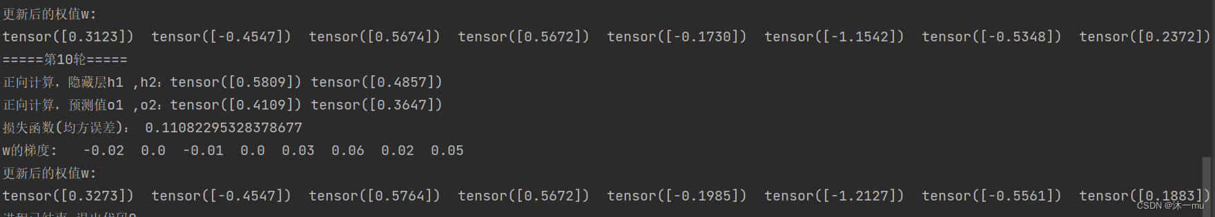
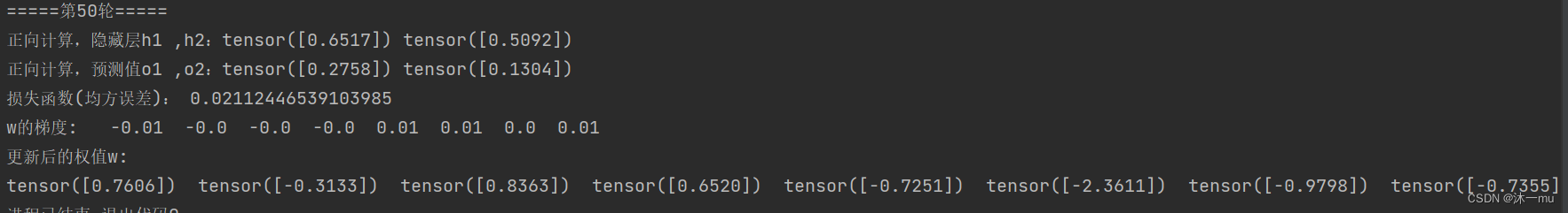
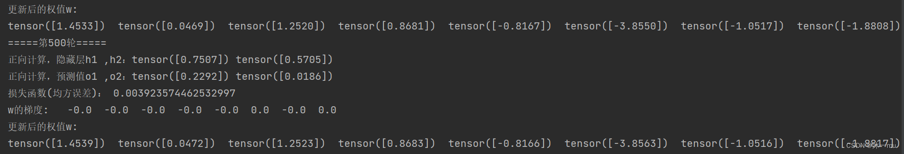
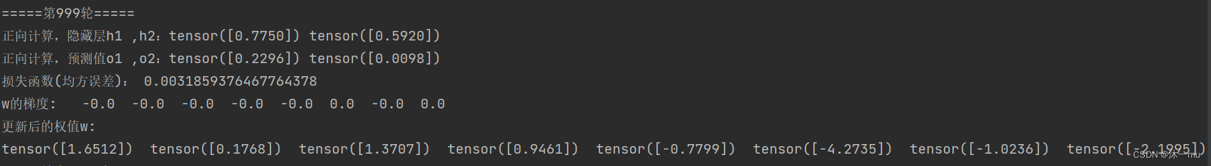
print("正向计算,隐藏层h1 ,h2:", end="")
print(out_h1.data, out_h2.data)
print("正向计算,预测值o1 ,o2:", end="")
print(out_o1.data, out_o2.data)
return out_o1, out_o2
def loss(x, y): # 损失函数
y_pre = forward_propagate(x) # 前向传播
#loss_mse = (1 / 2) * (y_pre[0] - y[0]) ** 2 + (1 / 2) * (y_pre[1] - y[1]) ** 2 # 考虑 : t.nn.MSELoss()
loss_mse1 = torch.nn.MSELoss()(y_pre[0],y[0])
loss_mse2 = torch.nn.MSELoss()(y_pre[1], y[1])
loss_mse = loss_mse1+loss_mse2
print("损失函数(均方误差):", loss_mse.item())
return loss_mse
if __name__ == "__main__":
for k in range(10):
print("\n=====第" + str(k+1) + "轮=====")
l = loss(x, y) # 前向传播,求 Loss,构建计算图
l.backward() # 反向传播,求出计算图中所有梯度存入w中. 自动求梯度,不需要人工编程实现。
print("w的梯度: ", end=" ")
for i in range(0, 8):
print(round(w[i].grad.item(), 2), end=" ") # 查看梯度
step = 1 # 步长
for i in range(0, 8):
w[i].data = w[i].data - step * w[i].grad.data # 更新权值
w[i].grad.data.zero_() # 注意:将w中所有梯度清零
print("\n更新后的权值w:")
for i in range(0, 8):
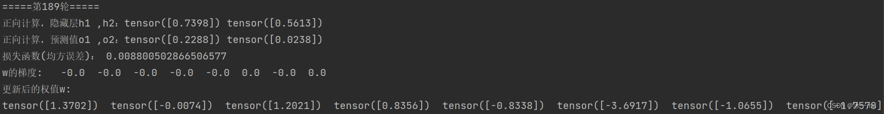
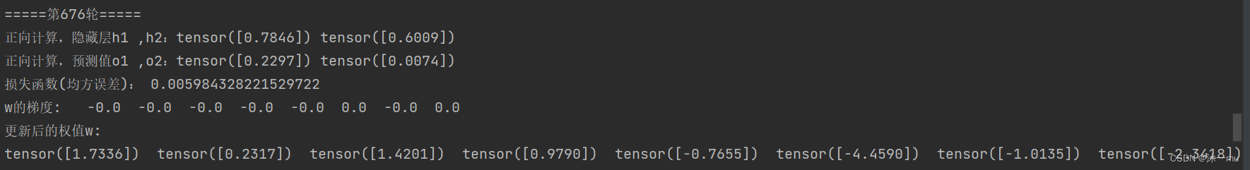
print(w[i].data, end=" ")执行结果:
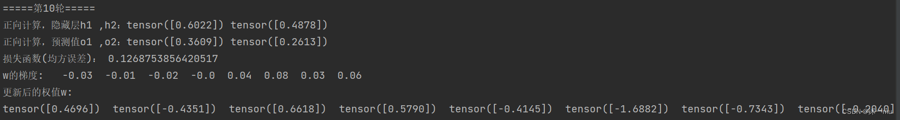
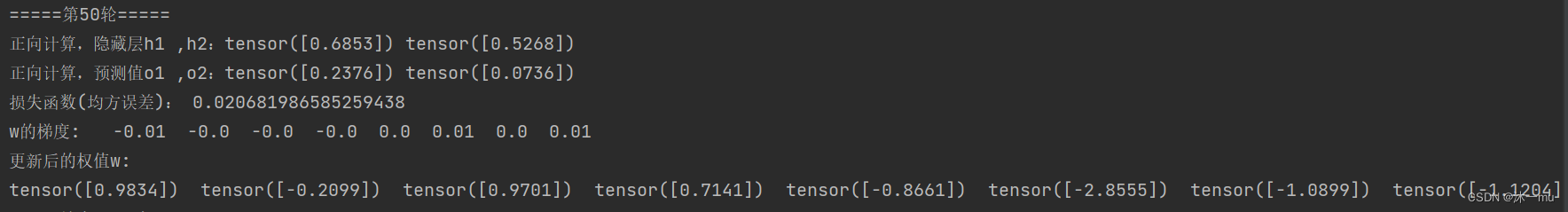

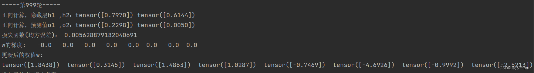
与之前的结果对比可以看出:在10轮时没更换之前的均方误差更低一些,在训练次数增多之后两个的训练结果就很接近了但手写的收敛结果也还是比直接调用torch.nn.MSELoss()要好一些。
5. 损失函数MSE改变为交叉熵
def loss_fuction(x1, x2, y1, y2):
    y1_pred, y2_pred = forward_propagate(x1, x2)
    loss_func = torch.nn.CrossEntropyLoss() # 创建交叉熵损失函数
    y_pred = torch.stack([y1_pred, y2_pred], dim=1)
    y = torch.stack([y1, y2], dim=1)
    loss = loss_func(y_pred, y) # 计算
    print("损失函数(交叉熵损失):", loss.item())
    return loss
执行结果:
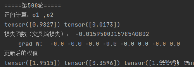
当训练轮数为500时,损失函数已经变为负的了。
- MSE 损失主要适用与回归问题,因为优化 MSE 等价于对高斯分布模型做极大似然估计,而简单回归中做服从高斯分布的假设是比较合理的
- 交叉熵损失主要适用于多分类问题,因为优化交叉熵损失等价于对多项式分布模型做极大似然估计,而多分类问题通常服从多项式分布
6. 改变步长,训练次数
import matplotlib.pyplot as plt
import torch

x1, x2 = torch.Tensor([0.5]), torch.Tensor([0.3])
y1, y2 = torch.Tensor([0.23]), torch.Tensor([-0.07])
print("=====输入值:x1, x2;真实输出值:y1, y2=====")
print(x1, x2, y1, y2)
w1, w2, w3, w4, w5, w6, w7, w8 = torch.Tensor([0.2]), torch.Tensor([-0.4]), torch.Tensor([0.5]), torch.Tensor(
    [0.6]), torch.Tensor([0.1]), torch.Tensor([-0.5]), torch.Tensor([-0.3]), torch.Tensor([0.8])  # 权重初始值
w1.requires_grad = True
w2.requires_grad = True
w3.requires_grad = True
w4.requires_grad = True
w5.requires_grad = True
w6.requires_grad = True
w7.requires_grad = True
w8.requires_grad = True

def sigmoid(z):
    a = 1 / (1 + torch.exp(-z))
    return a

def forward_propagate(x1, x2):
    in_h1 = w1 * x1 + w3 * x2
    out_h1 = sigmoid(in_h1)  # out_h1 = torch.sigmoid(in_h1)
    in_h2 = w2 * x1 + w4 * x2
    out_h2 = sigmoid(in_h2)  # out_h2 = torch.sigmoid(in_h2)

    in_o1 = w5 * out_h1 + w7 * out_h2
    out_o1 = sigmoid(in_o1)  # out_o1 = torch.sigmoid(in_o1)
    in_o2 = w6 * out_h1 + w8 * out_h2
    out_o2 = sigmoid(in_o2)  # out_o2 = torch.sigmoid(in_o2)

    print("正向计算:o1 ,o2")
    print(out_o1.data, out_o2.data)

    return out_o1, out_o2

def loss_fuction(x1, x2, y1, y2):  # 损失函数
    y1_pred, y2_pred = forward_propagate(x1, x2)  # 前向传播
    loss = (1 / 2) * (y1_pred - y1) ** 2 + (1 / 2) * (y2_pred - y2) ** 2  # 考虑 : t.nn.MSELoss()
    print("损失函数(均方误差):", loss.item())
    return loss

def update_w(w1, w2, w3, w4, w5, w6, w7, w8):
    # 步长
    step = 1
    w1.data = w1.data - step * w1.grad.data
    w2.data = w2.data - step * w2.grad.data
    w3.data = w3.data - step * w3.grad.data
    w4.data = w4.data - step * w4.grad.data
    w5.data = w5.data - step * w5.grad.data
    w6.data = w6.data - step * w6.grad.data
    w7.data = w7.data - step * w7.grad.data
    w8.data = w8.data - step * w8.grad.data
    w1.grad.data.zero_()  # 注意:将w中所有梯度清零
    w2.grad.data.zero_()
    w3.grad.data.zero_()
    w4.grad.data.zero_()
    w5.grad.data.zero_()
    w6.grad.data.zero_()
    w7.grad.data.zero_()
    w8.grad.data.zero_()
    return w1, w2, w3, w4, w5, w6, w7, w8

if __name__ == "__main__":

    print("=====更新前的权值=====")
    print(w1.data, w2.data, w3.data, w4.data, w5.data, w6.data, w7.data, w8.data)
    Y=[]
    X=[]

    for i in range(40):
        print("=====第" + str(i) + "轮=====")
        L = loss_fuction(x1, x2, y1, y2)  # 前向传播,求 Loss,构建计算图
        L.backward()  # 自动求梯度,不需要人工编程实现。反向传播,求出计算图中所有梯度存入w中
        print("\tgrad W: ", round(w1.grad.item(), 2), round(w2.grad.item(), 2), round(w3.grad.item(), 2),
              round(w4.grad.item(), 2), round(w5.grad.item(), 2), round(w6.grad.item(), 2), round(w7.grad.item(), 2),
              round(w8.grad.item(), 2))
        w1, w2, w3, w4, w5, w6, w7, w8 = update_w(w1, w2, w3, w4, w5, w6, w7, w8)
        Y.append(L.item())
        X.append(i)

    plt.rcParams['font.sans-serif'] = ['SimHei']  # 可以plt绘图过程中中文无法显示的问题
    plt.plot(X,Y)
    plt.xlabel('迭代次数')
    plt.ylabel('Loss,step=1')
    plt.show()
    print("更新后的权值")
    print(w1.data, w2.data, w3.data, w4.data, w5.data, w6.data, w7.data, w8.data)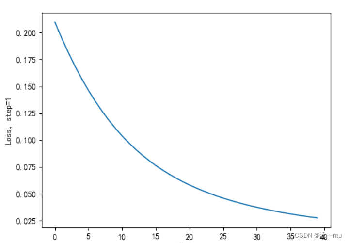
7.权值w1-w8初始值换为随机数,对比“指定权值”的结果
w1, w2, w3, w4, w5, w6, w7, w8 = torch.randn(1), torch.randn(1), torch.randn(1), torch.randn(1), \
torch.randn(1), torch.randn(1), torch.randn(1), torch.randn(1)=====输入值:x1, x2;真实输出值:y1, y2=====
tensor([0.5000]) tensor([0.3000]) tensor([0.2300]) tensor([-0.0700])
=====更新前的权值=====
tensor([-0.3827]) tensor([1.1477]) tensor([0.3640]) tensor([0.4843]) tensor([-0.6357]) tensor([0.6936]) tensor([-0.2005]) tensor([-0.0979])
=====第0轮=====
正向计算:o1 ,o2
tensor([0.3918]) tensor([0.5663])
损失函数(均方误差): 0.215525820851326
grad W: 0.01 -0.0 0.01 -0.0 0.02 0.07 0.03 0.11
更新后的权值
tensor([-0.3931]) tensor([1.1503]) tensor([0.3577]) tensor([0.4858]) tensor([-0.6542]) tensor([0.6187]) tensor([-0.2265]) tensor([-0.2030])改变随机数值,改变了权值,但对收敛速度基本没有影响。
8.权值w1-w8初始值换为0
w1, w2, w3, w4, w5, w6, w7, w8 = torch.Tensor([0]), torch.Tensor([0]), torch.Tensor([0]), torch.Tensor(
    [0]), torch.Tensor([0]), torch.Tensor([0]), torch.Tensor([0]), torch.Tensor([0])
神经网络用的是梯度下降法,来进行每次更新网络的权重w,假如loss函数为: (简写的)
Loss = (y - y’)^2, 其中y = f(wx + b)
那么,每次更新w用求导法则 w = w + w’, w’ = (Loss对w的求导)
w’ 应该是:(Loss对y求导)(y对f函数求导)(f函数对w求导)2. 注意上述中间项:(y对f型函数求导)
9.体会
通过这次作业的学习我对BP算法有了更深的理解,也调了很多参数函数等等,当然在过程中也遇到了一些困难,例如在损失函数MSE用PyTorch自带函数 t.nn.MSELoss()替代过程中,执行过程中一直报错,找了其他同学的博客也没有很好的解决,最后还是请教了大佬成功解决了问题。不仅仅是在作业中在生活中也是有了一些波折,这次河大的疫情来的很突然,希望每个人都能遵守好学校的纪律共度难关。
ref:
【2021-2022 春学期】人工智能-作业2:例题程序复现_HBU_David的博客-CSDN博客
【2021-2022 春学期】人工智能-作业3:例题程序复现 PyTorch版_HBU_David的博客-CSDN博客
【人工智能导论:模型与算法】MOOC 8.3 误差后向传播(BP) 例题 编程验证 Pytorch版本 - HBU_DAVID - 博客园
【人工智能导论:模型与算法】MOOC 8.3 误差后向传播(BP) 例题 【第三版】 - HBU_DAVID - 博客园


 被折叠的 条评论
为什么被折叠?
被折叠的 条评论
为什么被折叠?
 到【灌水乐园】发言


