深度学习作业7_证明宽卷积具有交换性-CSDN博客

本文链接：https://blog.csdn.net/m0_64715292/article/details/127604447

习题5-4 对于一个输入为100×100×256的特征映射组，使用3×3的卷积核，输出为100×100×256的特征映射组的卷积层，求其时间和空间复杂度。如果引入一个1×1的卷积核，先得到100×100×64的特征映射，再进行3×3的卷积，得到100×100×256的特征映射组，求其时间和空间复杂度。

习题5-7 忽略激活函数，分析卷积网络中卷积层的前向计算和反向传播是一种转置关系。

选做推导CNN反向传播算法

选做pyorch实现卷积层和池化层反向传播算子

ref

习题5-2 证明宽卷积具有交换性

首先，宽卷积定义为，其中 $\widetilde{\otimes }$ 表示宽卷积运算，我们不妨先设一个二维图像 $X\in R^{M\times N}$ 和一个二维卷积核 $W=R^{U\times V}$ ,然后对该二维图像X进行零填充，两端各补U-1 和V-1 个零，得到全填充的图像 $\widetilde{X}\in R^{(M+2U-2)\times (N+2V-2)}$

现有

$y_{ij}=\sum^m_{u=1}\sum^n_{v=1}w_{uv}\cdot x_{i+u-1,j+v-1}$

根据宽卷积定义

$y_{ij}=\sum^m_{n=1-(m-1)}\sum^n_{v=1-(n-1)}w_{uv}\cdot x_{i+u-1,j+v-1}$

为了让x的下标形式和w的进行对换，进行变量替换

令 $s=i-u+1, t=j-v+1$ , 故 $u=s-i+1,v=t-j+1$

则

$y_{ij}=\sum^{i-1+m}_{s=i+1-m}\sum^{j-1+n}_{t=j+1-n}x_{st}\cdot w_{s-i+1,t-j+1}$

已知 $i \in [1,M]J,J \in [1,N]$

因此对于

$y_{ij}=\sum^{i-1+m}_{s=i+1-m}\sum^{j-1+n}_{t=j+1-n}x_{st}w_{s-i+1,t-j+1}$

由于宽卷积的条件，s和t的变动范围是可行的。

习题5-3 分析卷积神经网络中1 $\times$ 1卷积核的作用

升维降维

1*1卷积是大小为1*1的滤波器做卷积操作，不同于2*2、3*3等filter，没有考虑在前一特征层局部信息之间的关系。升维是用最少的参数拓宽网络，降维缩减网络通道数，减少参数，减少计算量。

增加非线性特性

1*1卷积核，可以在保持特征图尺度不变的（即不损失分辨率）的前提下大幅增加非线性特性（利用后接的非线性激活函数），把网络做的很深。备注：一个卷积核对应卷积后得到一个特征图，不同的卷积权重，卷积以后得到不同的特征图，提取不同的特征。

跨通道信息互换（channal的变换）

GoogLeNet利用1×1的卷积降维后，得到了更为紧凑的网络结构，虽然总共有22层，但是参数数量却只是8层的AlexNet的十二分之一。

习题5-4 对于一个输入为100×100×256的特征映射组，使用3×3的卷积核，输出为100×100×256的特征映射组的卷积层，求其时间和空间复杂度。如果引入一个1×1的卷积核，先得到100×100×64的特征映射，再进行3×3的卷积，得到100×100×256的特征映射组，求其时间和空间复杂度。

3×3

时间复杂度： $O_{times}(M^2*K^2*C_{in}*C_{out})=256\times 100\times 100\times 256\times 3\times 3=5898240000$

空间复杂度： $O_{space}(M^2*K^2*C_{in}*C_{out})=256\times 100\times 100=2560000$

1×1

时间复杂度：

$O_{times}(M^2*K^2*C_{in}*C_{out})=256\times 100\times 100\times 64+256\times 100\times 100\times 64\times 3\times 3=1638400000$

空间复杂度: $O_{space}(M^2*K^2*C_{in}*C_{out})=64\times 100\times 100+256\times 100\times 100=3200000$

习题5-7 忽略激活函数，分析卷积网络中卷积层的前向计算和反向传播是一种转置关系。

以一个3×3的卷积核为例，输入为X输出为Y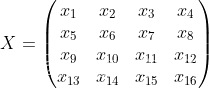
在这里插入图片描述 $X=\begin{pmatrix} x_1&x_2&x_3&x_4\ x_5&x_6&x_7&x_8\ x_9&x_{10}&x_{11}&x_{12}\ x_{13}&x_{14}&x_{15}&x_{16}\ \end{pmatrix}W=\begin{pmatrix} w_{00}&w_{01}&w_{02}\ w_{10}&w_{11}&w_{12}\ w_{20}&w_{21}&w_{22}\ \end{pmatrix}Y=\begin{pmatrix} y_1&y_2\ y_3&y_4\ \end{pmatrix}$

将4×4的输入特征展开为16×1的矩阵，y展开为4×1的矩阵，将卷积计算转化为矩阵相乘
在这里插入图片描述

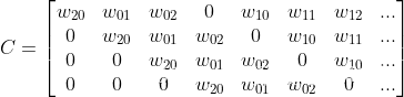
由
而
即
所以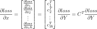

综上可以看出前向计算和反向传播是一种转置关系。

选做推导CNN反向传播算法

CNN主要分为汇聚层（池化层）和卷积层反向传播的推导

其中池化层的反向传播比较容易理解，以最大池化举例，如下图，池化后的数字6对应于池化前的红色区域，实际上只有红色区域中最大值数字6对池化后的结果有影响，权重为1，而其它的数字对池化后的结果影响都为0。假设池化后数字6的位置delta误差为，误差反向传播回去时，红色区域中最大值对应的位置delta误差即等于，而其它3个位置对应的delta误差为0。

因此，在卷积神经网络最大池化前向传播时，不仅要记录区域的最大值，同时也要记录下来区域最大值的位置，方便delta误差的反向传播。

而平均池化就更简单了，由于平均池化时，区域中每个值对池化后结果贡献的权重都为区域大小的倒数，所以delta误差反向传播回来时，在区域每个位置的delta误差都为池化后delta误差除以区域的大小。

然后卷积层就是通过张量卷积，或者说若干个矩阵卷积求和而得到当前层的输出，这和一般的网络直接进行矩阵乘法得到当前层的输出不同。这样在卷积层反向传播的时候，上一层误差的递推计算方法肯定有所不同。
对于卷积层，由于W使用的运算是卷积，那么由该层误差推导出该层的所有卷积核的W,b的方式也不同。由于卷积层可以有多个卷积核，各个卷积核的处理方法是完全相同且独立的。

选做pyorch实现卷积层和池化层反向传播算子

卷积层：

from typing import Dict, Tuple
import numpy as np
import pytest
import torch
 
def conv2d_forward(input: np.ndarray, weight: np.ndarray, bias: np.ndarray,
                   stride: int, padding: int) -> Dict[str, np.ndarray]:
    """2D Convolution Forward Implemented with NumPy
    Args:
        input (np.ndarray): The input NumPy array of shape (H, W, C).
        weight (np.ndarray): The weight NumPy array of shape
            (C', F, F, C).
        bias (np.ndarray | None): The bias NumPy array of shape (C').
            Default: None.
        stride (int): Stride for convolution.
        padding (int): The count of zeros to pad on both sides.
    Outputs:
        Dict[str, np.ndarray]: Cached data for backward prop.
    """
    h_i, w_i, c_i = input.shape
    c_o, f, f_2, c_k = weight.shape
 
    assert (f == f_2)
    assert (c_i == c_k)
    assert (bias.shape[0] == c_o)
    input_pad = np.pad(input, [(padding, padding), (padding, padding), (0, 0)])
 
    def cal_new_sidelngth(sl, s, f, p):
        return (sl + 2 * p - f) // s + 1
 
    h_o = cal_new_sidelngth(h_i, stride, f, padding)
    w_o = cal_new_sidelngth(w_i, stride, f, padding)
    output = np.empty((h_o, w_o, c_o), dtype=input.dtype)
 
    for i_h in range(h_o):
        for i_w in range(w_o):
            for i_c in range(c_o):
                h_lower = i_h * stride
                h_upper = i_h * stride + f
                w_lower = i_w * stride
                w_upper = i_w * stride + f
                input_slice = input_pad[h_lower:h_upper, w_lower:w_upper, :]
                kernel_slice = weight[i_c]
                output[i_h, i_w, i_c] = np.sum(input_slice * kernel_slice)
                output[i_h, i_w, i_c] += bias[i_c]
 
    cache = dict()
    cache['Z'] = output
    cache['W'] = weight
    cache['b'] = bias
    cache['A_prev'] = input
    return cache
 
def conv2d_backward(dZ: np.ndarray, cache: Dict[str, np.ndarray], stride: int,
                    padding: int) -> Tuple[np.ndarray, np.ndarray, np.ndarray]:
    """2D Convolution Backward Implemented with NumPy
    Args:
        dZ: (np.ndarray): The derivative of the output of conv.
        cache (Dict[str, np.ndarray]): Record output 'Z', weight 'W', bias 'b'
            and input 'A_prev' of forward function.
        stride (int): Stride for convolution.
        padding (int): The count of zeros to pad on both sides.
    Outputs:
        Tuple[np.ndarray, np.ndarray, np.ndarray]: The derivative of W, b,
            A_prev.
    """
    W = cache['W']
    b = cache['b']
    A_prev = cache['A_prev']
    dW = np.zeros(W.shape)
    db = np.zeros(b.shape)
    dA_prev = np.zeros(A_prev.shape)
 
    _, _, c_i = A_prev.shape
    c_o, f, f_2, c_k = W.shape
    h_o, w_o, c_o_2 = dZ.shape
 
    assert (f == f_2)
    assert (c_i == c_k)
    assert (c_o == c_o_2)
 
    A_prev_pad = np.pad(A_prev, [(padding, padding), (padding, padding),
                                 (0, 0)])
    dA_prev_pad = np.pad(dA_prev, [(padding, padding), (padding, padding),
                                   (0, 0)])
    for i_h in range(h_o):
        for i_w in range(w_o):
            for i_c in range(c_o):
                h_lower = i_h * stride
                h_upper = i_h * stride + f
                w_lower = i_w * stride
                w_upper = i_w * stride + f
 
                input_slice = A_prev_pad[h_lower:h_upper, w_lower:w_upper, :]
                # forward
                # kernel_slice = W[i_c]
                # Z[i_h, i_w, i_c] = np.sum(input_slice * kernel_slice)
                # Z[i_h, i_w, i_c] += b[i_c]
 
                # backward
                dW[i_c] += input_slice * dZ[i_h, i_w, i_c]
                dA_prev_pad[h_lower:h_upper,
                            w_lower:w_upper, :] += W[i_c] * dZ[i_h, i_w, i_c]
                db[i_c] += dZ[i_h, i_w, i_c]
 
    if padding > 0:
        dA_prev = dA_prev_pad[padding:-padding, padding:-padding, :]
    else:
        dA_prev = dA_prev_pad
    return dW, db, dA_prev
 
@pytest.mark.parametrize('c_i, c_o', [(3, 6), (2, 2)])
@pytest.mark.parametrize('kernel_size', [3, 5])
@pytest.mark.parametrize('stride', [1, 2])
@pytest.mark.parametrize('padding', [0, 1])
def test_conv(c_i: int, c_o: int, kernel_size: int, stride: int, padding: str):
 
    # Preprocess
    input = np.random.randn(20, 20, c_i)
    weight = np.random.randn(c_o, kernel_size, kernel_size, c_i)
    bias = np.random.randn(c_o)
 
    torch_input = torch.from_numpy(np.transpose(
        input, (2, 0, 1))).unsqueeze(0).requires_grad_()
    torch_weight = torch.from_numpy(np.transpose(
        weight, (0, 3, 1, 2))).requires_grad_()
    torch_bias = torch.from_numpy(bias).requires_grad_()
 
    # forward
    torch_output_tensor = torch.conv2d(torch_input, torch_weight, torch_bias,
                                       stride, padding)
    torch_output = np.transpose(
        torch_output_tensor.detach().numpy().squeeze(0), (1, 2, 0))
 
    cache = conv2d_forward(input, weight, bias, stride, padding)
    numpy_output = cache['Z']
    assert np.allclose(torch_output, numpy_output)
 
    # backward
    torch_sum = torch.sum(torch_output_tensor)
    torch_sum.backward()
    torch_dW = np.transpose(torch_weight.grad.numpy(), (0, 2, 3, 1))
    torch_db = torch_bias.grad.numpy()
    torch_dA_prev = np.transpose(torch_input.grad.numpy().squeeze(0),
                                 (1, 2, 0))
 
    dZ = np.ones(numpy_output.shape)
    dW, db, dA_prev = conv2d_backward(dZ, cache, stride, padding)
 
    assert np.allclose(dW, torch_dW)
    assert np.allclose(db, torch_db)
    assert np.allclose(dA_prev, torch_dA_prev)

池化层:

import numpy as np
from module import Layers 
 
class Pooling(Layers):
    def __init__(self, name, ksize, stride, type):
        super(Pooling).__init__(name)
        self.type = type
        self.ksize = ksize
        self.stride = stride 
 
    def forward(self, x):
        b, c, h, w = x.shape
        out = np.zeros([b, c, h//self.stride, w//self.stride]) 
        self.index = np.zeros_like(x)
        for b in range(b):
            for d in range(c):
                for i in range(h//self.stride):
                    for j in range(w//self.stride):
                        _x = i *self.stride
                        _y = j *self.stride
                        if self.type =="max":
                            out[b, d, i, j] = np.max(x[b, d, _x:_x+self.ksize, _y:_y+self.ksize])
                            index = np.argmax(x[b, d, _x:_x+self.ksize, _y:_y+self.ksize])
                            self.index[b, d, _x +index//self.ksize, _y +index%self.ksize ] = 1
                        elif self.type == "aveg":
                            out[b, d, i, j] = np.mean((x[b, d, _x:_x+self.ksize, _y:_y+self.ksize]))
        return out 
 
    def backward(self, grad_out):
        if self.type =="max":
            return np.repeat(np.repeat(grad_out, self.stride, axis=2),self.stride, axis=3)* self.index 
        elif self.type =="aveg":
            return np.repeat(np.repeat(grad_out, self.stride, axis=2), self.stride, axis=3)/(self.ksize * self.ksize)