实验《MATLAB绘图操作》

1.绘制函数曲线

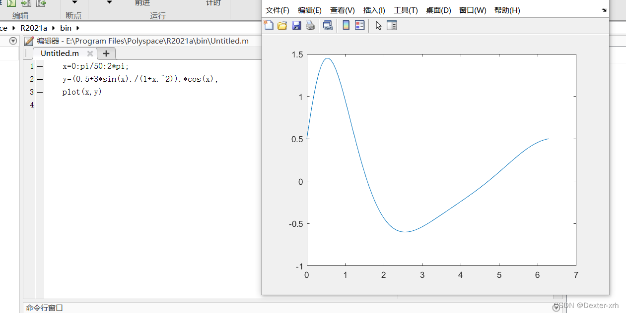
（1）绘制函数曲线。设,把x=0~2π区间分为101点，绘制函数的曲线。

x=0:pi/50:2*pi;

y=(0.5+3*sin(x)./(1+x.^2)).*cos(x);

plot(x,y)

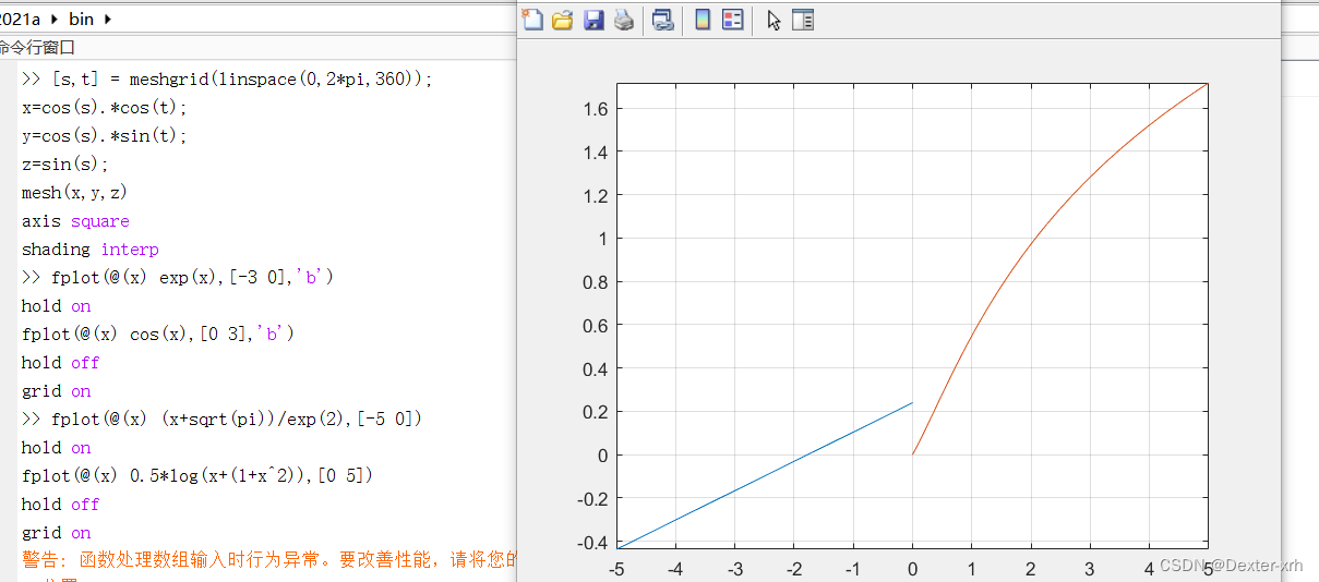
（2） 已知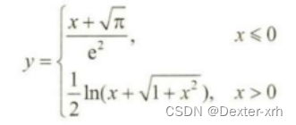在-5<xs5 区间绘制函数曲线

fplot(@(x) (x+sqrt(pi))/exp(2),[-5 0])

hold on

fplot(@(x) 0.5*log(x+(1+x^2)),[0 5])

hold off

grid on

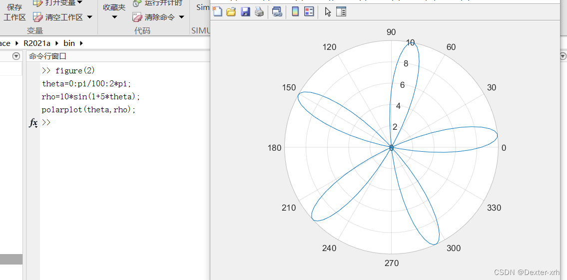
 (3)绘制极坐标曲线 p=10sin(1+50)。

figure(2)

theta=0:pi/100:2*pi;

rho=10*sin(1+5*theta);

polarplot(theta,rho);

2.已知 yi=x2，y2=cos(2x)，y3=y1*y2，完成下列操作。

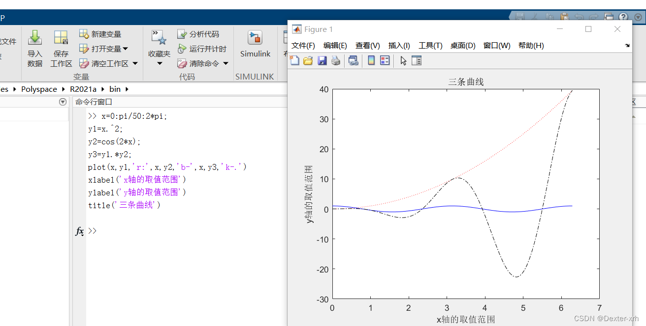
(1)在同一坐标系下用不同的颜色和线型绘制 3 条曲线

 x=0:pi/50:2*pi;

y1=x.^2;

y2=cos(2*x);

y3=y1.*y2;

plot(x,y1,'r:',x,y2,'b-',x,y3,'k-.')

xlabel('x轴的取值范围')

ylabel('y轴的取值范围')

title('三条曲线')

 
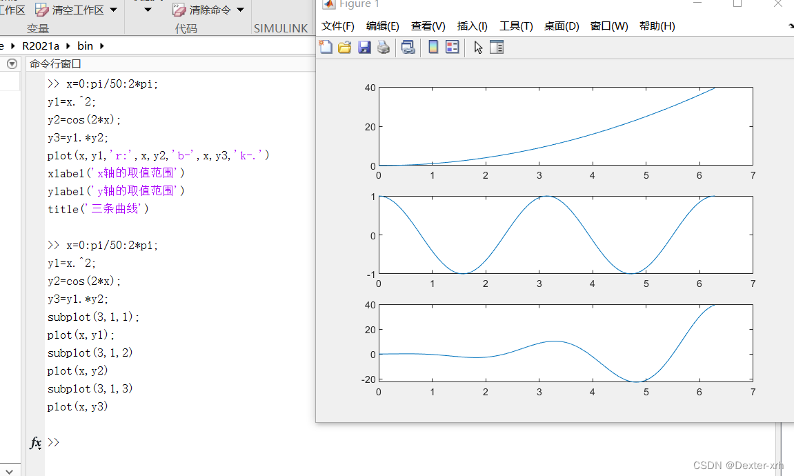
(2)以子图形式绘制 3 条曲线。

x=0:pi/50:2*pi;

y1=x.^2;

y2=cos(2*x);

y3=y1.*y2;

subplot(3,1,1);

plot(x,y1);

subplot(3,1,2)

plot(x,y2)

subplot(3,1,3)

plot(x,y3)

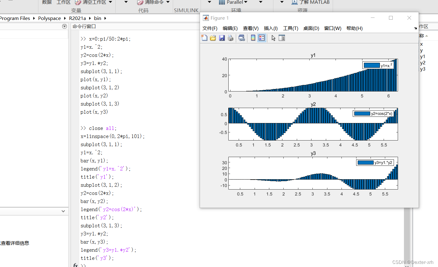
(3) 分别用条形图、阶梯图、杆图和填充图绘制 3 条曲线 

close all;

x=linspace(0,2*pi,101);

subplot(3,1,1);

y1=x.^2;

bar(x,y1);

legend('y1=x.^2');

title('y1');

subplot(3,1,2);

y2=cos(2*x);

bar(x,y2);

legend('y2=cos(2*x)');

title('y2');

subplot(3,1,3);

y3=y1.*y2;

bar(x,y3);

legend('y3=y1.*y2');

title('y3');

4.绘制函数的曲面图和等高线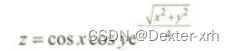
其中 x 的 21 个值均匀分布在[-5,5]范围，的 31 个值均分布在[010]，要求使用subplot(2,1,1)和 subplot(2,1,2)将产生的曲面图和等高线图画在同一个窗口上。

x=linspace(-5,5,21);

y=linspace(0,10,31);

[xx,yy]=meshgrid(x,y);

zz=cos(xx).*cos(yy).*exp(-sqrt(xx.^2+yy.^2)/4);

subplot(1,2,1)%我感觉竖着放不如横着放好看，就横放了，

              %如果按要求是要用subplot(2,1,1),

              %下面也相应改成subplot(2,1,2)

surf(xx,yy,zz)

xlabel('x'),ylabel('y'),zlabel('z')

subplot(1,2,2)

contour(xx,yy,zz,21),axis square

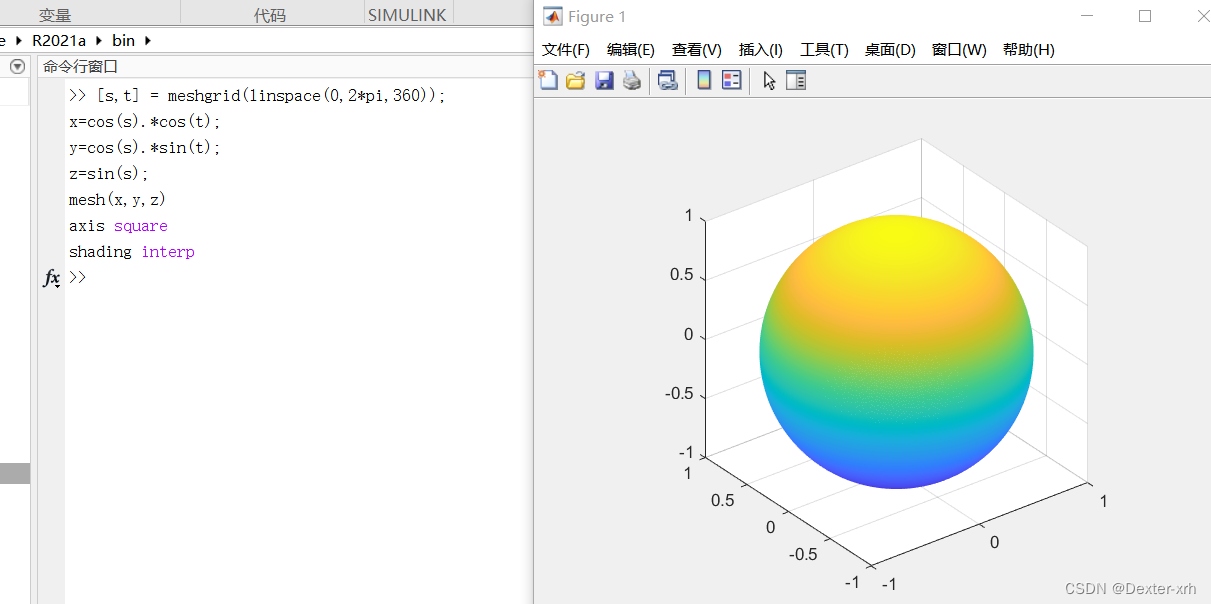
5.绘制曲面图形，并进行插值着色处理。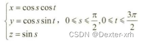

[s,t] = meshgrid(linspace(0,2*pi,360));

x=cos(s).*cos(t);

y=cos(s).*sin(t);

z=sin(s);

mesh(x,y,z)

axis square

shading interp