2 Classification Overview

2. Classification Overview

Click here for notes and code

MNIST

Initial Knowledge Dataset

MNIST dataset is a set of 70,000 small images of digits handwritten by high school students and employees of the US Census Bureau. Each image is labeled with the digit it represents.

The following code fetches the MNIST dataset:

>>> from sklearn.datasets import fetch_openml
>>> mnist = fetch_openml('mnist_784', version=1)
>>> mnist.keys()
dict_keys(['data', 'target', 'feature_names', 'DESCR', 'details',
 'categories', 'url'])

Datasets loaded by Scikit-Learn generally have a similar dictionary structure includ‐
ing:

• A DESCR key describing the dataset
• A data key containing an array with one row per instance and one column per feature
• A target key containing an array with the labels

>>> X, y = mnist["data"], mnist["target"]
>>> X.shape
(70000, 784)
>>> y.shape
(70000,)

• There are 70,000 images, and each image has 784 features.
• This is because each image is 28×28=784 pixels, and each feature simply represents one pixel’s intensity, from 0 (white) to 255 (black).

Let’s take a peek at one digit from the dataset.

All you need to do is grab an instance’s feature vector, reshape it to a 28×28 array, and display it .

import matplotlib as mpl
import matplotlib.pyplot as plt

some_digit = X[0]
some_digit_image = some_digit.reshape(28, 28)

plt.imshow(some_digit_image, cmap = mpl.cm.binary)
plt.show()

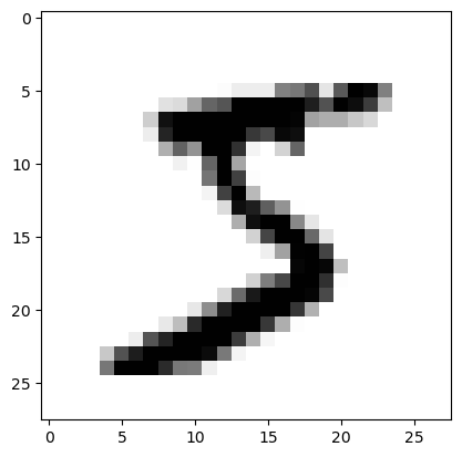
This looks like a 5, and indeed that’s what the label tells us:

>>> y[0]
'5'

Note that the label is a string. We prefer numbers, so let’s cast y to integers:

>>> y = y.astype(np.uint8)

Train Set And Test Set

The MNIST dataset is actually already split into a training set (the first 60,000
images) and a test set (the last 10,000 images):

X_train, X_test, y_train, y_test = X[:60000], X[60000:], y[:60000], y[60000:]

• The training set is already shuffled for us, which is good as this guarantees that all cross-validation folds will be similar.
• Moreover, some learning algorithms are sensitive to the order of the training instances, and they perform poorly if they get many similar instances in a row.

Training a Binary Classifier

Now only try to identify one digit—the number 5.

Create the target vectors for this classification task.

y_train_5 = (y_train == 5) # True for all 5s, False for all other digits.
y_test_5 = (y_test == 5)

A good place to start is with a Stochastic Gradient Descent (SGD) classifier, using Scikit-Learn’s SGDClassifier class. This classifier has the advantage of being capable of handling very large datasets efficiently

from sklearn.linear_model import SGDClassifier
sgd_clf = SGDClassifier(random_state=42)
sgd_clf.fit(X_train, y_train_5)

The SGDClassifier relies on randomness during training (hence the name “stochastic”). If you want reproducible results, you should set the random_state parameter.

Use it to detect images of the number 5

>>> sgd_clf.predict([some_digit])
array([ True])

Performance Measures

Measuring Accuracy Using Cross-Validation

>>> from sklearn.model_selection import cross_val_score
>>> cross_val_score(sgd_clf, X_train, y_train_5, cv=3, scoring="accuracy")
array([0.96355, 0.93795, 0.95615])

Above 93% accuracy (ratio of correct predictions) on all cross-validation folds. This looks amazing. In fact, this is simply because only about 10% of the images are 5s, so if you always guess that an image is not a 5, you will be right about 90% of the time.

This demonstrates why accuracy is generally not the preferred performance measure for classifiers, especially when you are dealing with skewed datasets (i.e., when some classes are much more frequent than others).

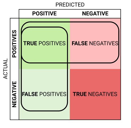
Confusion Matrix

A much better way to evaluate the performance of a classifier is to look at the confusion matrix. The general idea is to count the number of times instances of class A are classified as class B.

For example, to know the number of times the classifier confused images of 5s with 3s, you would look in the 5th row and 3rd column of the confusion matrix.

cross_val_predict() performs K-fold cross-validation, and it returns the predictions made on each test fold.

from sklearn.model_selection import cross_val_predict
y_train_pred = cross_val_predict(sgd_clf, X_train, y_train_5, cv=3)

Get the confusion matrix.

>>> from sklearn.metrics import confusion_matrix
>>> confusion_matrix(y_train_5, y_train_pred)
array([[53057, 1522],
			 [ 1325, 4096]])

Each row in a confusion matrix represents an actual class, while each column represents a predicted class.

• The first row of this matrix considers non-5 images (the negative class): 53,057 of them were correctly classified as non-5s (they are called true negatives), while the remaining 1,522 were wrongly classified as 5s (false positives).
• The second row considers the images of 5s (the positive class): 1,325 were wrongly classified as non-5s (false negatives), while the remaining 4,096 were correctly classified as 5s (true positives).
• A perfect classifier would have only true positives and true negatives, so its confusion matrix would have nonzero values only on its main diagonal (top left to bottom right):

>>> y_train_perfect_predictions = y_train_5 # pretend we reached perfection
>>> confusion_matrix(y_train_5, y_train_perfect_predictions)
array([[54579, 0],
			 [ 0, 5421]])

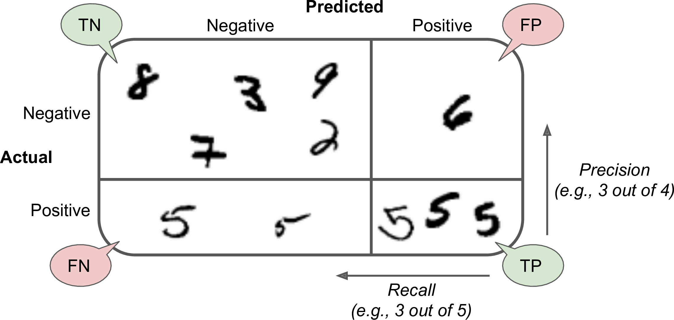
Precision and Recall

precision

$$
\text{precision }= \dfrac{TP}
{TP

• FP}
  $$

• TP is the number of true positives, and FP is the number of false positives.

recall (sensitivity / true positive rate (TPR))

$$
\text{recall}=\dfrac{TP}
{TP

• FN}
  $$

• FN is of course the number of false negatives.

Scikit-Learn provides several functions to compute classifier metrics, including preci‐
sion and recall:

>>> from sklearn.metrics import precision_score, recall_score
>>> precision_score(y_train_5, y_train_pred) # == 4096 / (4096 + 1522)
0.7290850836596654
>>> recall_score(y_train_5, y_train_pred) # == 4096 / (4096 + 1325)
0.7555801512636044

Now your 5-detector does not look as shiny as it did when you looked at its accuracy.
When it claims an image represents a 5, it is correct only 72.9% of the time. Moreover, it only detects 75.6% of the 5s.

It is often convenient to combine precision and recall into a single metric called the F1

score, in particular if you need a simple way to compare two classifiers. The F1score is the harmonic mean of precision and recall.

$$F_1=\frac{2}{\frac{1}{\text{ precision }}+\frac{1}{\text{ recall }}}=2\times \frac{\text{ precision }\times \text{ recall }}{\text{ precision }+\text{ recall }}=\frac{TP}{TP+\frac{FN+FP}{2}}$$

To compute the F1score, simply call the f1_score() function:

>>> from sklearn.metrics import f1_score
>>> f1_score(y_train_5, y_train_pred)
0.7420962043663375

• The F1 score favors classifiers that have similar precision and recall. This is not always
  what you want: in some contexts you mostly care about precision, and in other contexts you really care about recall.
  • detect videos that are safe for kids→high precision
  • detect shoplifters on surveillance images→high recall
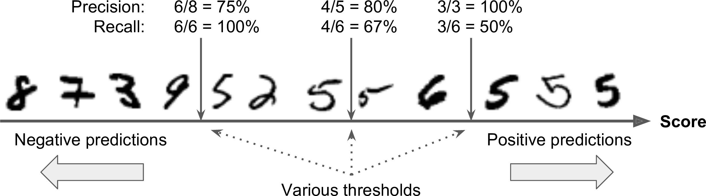
• Precision and recall cannot increase at the same time, this is called the precision/recall tradeoff.

Precision/Recall Tradeof

For each instance, the SGDClassifier computes a score based on a decision function, and if that score is greater than a threshold, it assigns the instance to the positive class, or else it assigns it to the negative class.

Scikit-Learn does not let you set the threshold directly, but it does give you access to
the decision scores that it uses to make predictions.

You can call its decision_function()method, which returns a score for each instance, and then make predictions based on those scores using any threshold you want:

>>> y_scores = sgd_clf.decision_function([some_digit])
>>> y_scores
array([2412.53175101])
>>> threshold = 0
>>> y_some_digit_pred = (y_scores > threshold)
array([ True])

The SGDClassifier uses a threshold equal to 0, so the previous code returns the same
result as the predict() method (i.e., True). Let’s raise the threshold:

>>> threshold = 8000
>>> y_some_digit_pred = (y_scores > threshold)
>>> y_some_digit_pred
array([False])

This confirms that raising the threshold decreases recall. The image actually represents a 5, and the classifier detects it when the threshold is 0, but it misses it when the threshold is increased to 8,000.

How do you decide which threshold to use?

For this you will first need to get the scores of all instances in the training set using the cross_val_predict() function again.

>>> y_scores = cross_val_predict(sgd_clf, X_train, y_train_5, cv=3,
																 method="decision_function")

Now with these scores you can compute precision and recall for all possible thresholds using the precision_recall_curve() function:

from sklearn.metrics import precision_recall_curve
precisions, recalls, thresholds = precision_recall_curve(y_train_5, y_scores)

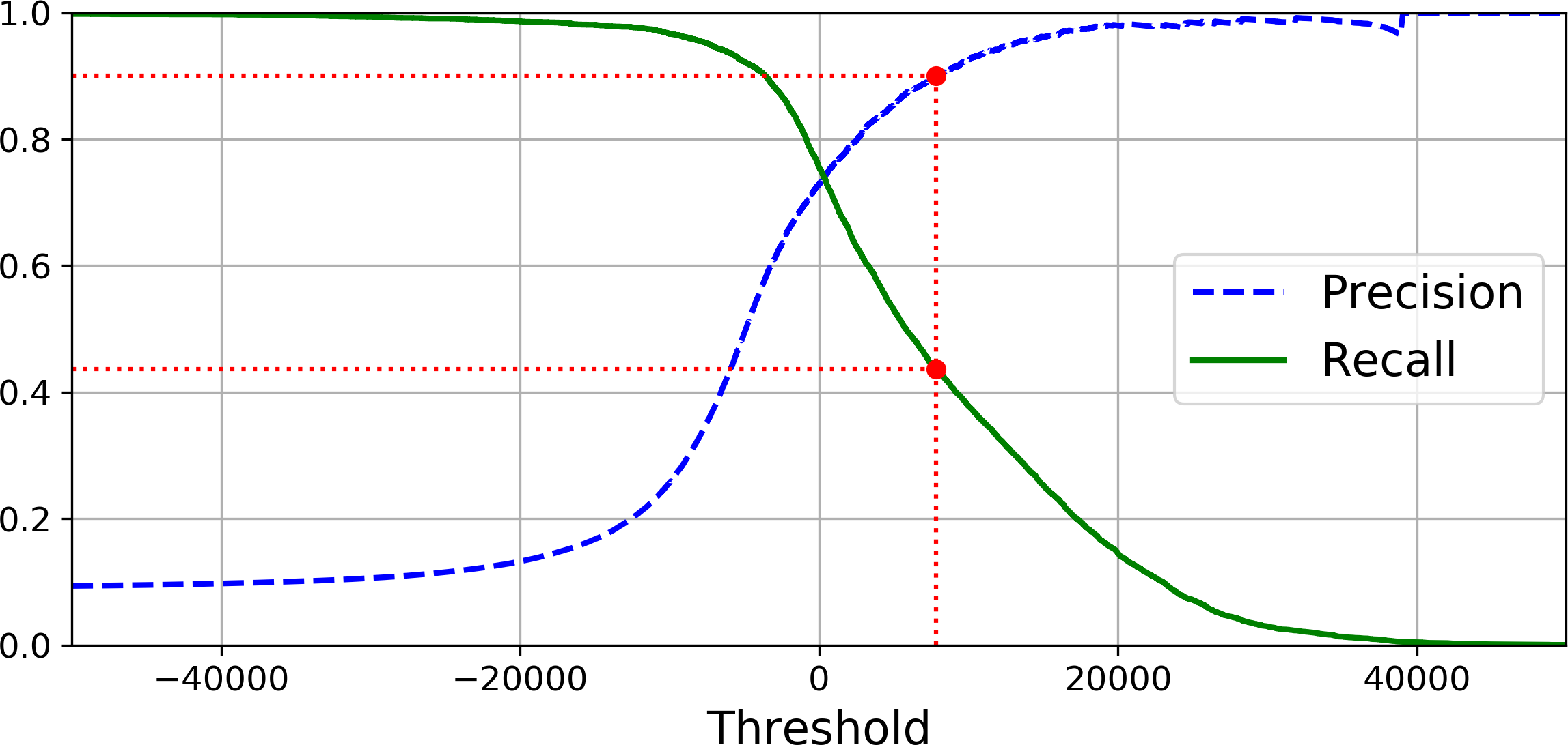
Finally, you can plot precision and recall as functions of the threshold value using
Matplotlib:

def plot_precision_recall_vs_threshold(precisions, recalls, thresholds):
 plt.plot(thresholds, precisions[:-1], "b--", label="Precision")
 plt.plot(thresholds, recalls[:-1], "g-", label="Recall")
 [...] # highlight the threshold, add the legend, axis label and grid
plot_precision_recall_vs_threshold(precisions, recalls, thresholds)
plt.show()

Another way to select a good precision/recall tradeoff is to plot precision directly against recall.

• Pprecision really starts to fall sharply around 80% recall.
• Probably select a precision/recall tradeoff just before that drop.

Suppose to aim for 90% precision.

>>> threshold_90_precision = thresholds[np.argmax(precisions >= 0.90)]
7816

Let’s check these predictions’ precision and recall:

>>> precision_score(y_train_5, y_train_pred_90)
0.9000380083618396
>>> recall_score(y_train_5, y_train_pred_90)
0.4368197749492714

If someone says “let’s reach 99% precision,” you should ask, “at what recall?”

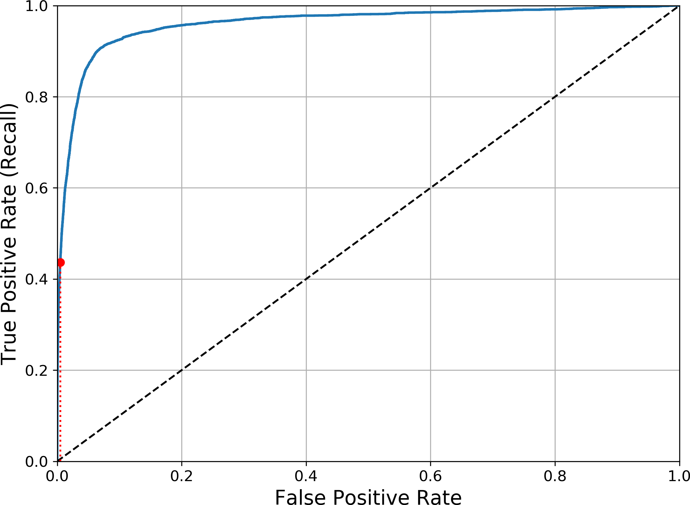
The ROC Curve

The receiver operating characteristic (ROC) curve is another common tool used with binary classifiers.

The ROC curve plots the true positive rate (another name for recall) against the false positive rate.

$$TPR=\frac{TP}{P}=\frac{TP}{TP+FN}=1-FNR$$

$$FNR=\frac{FN}{P}=\frac{TP}{TP+FN}=1-TPR$$

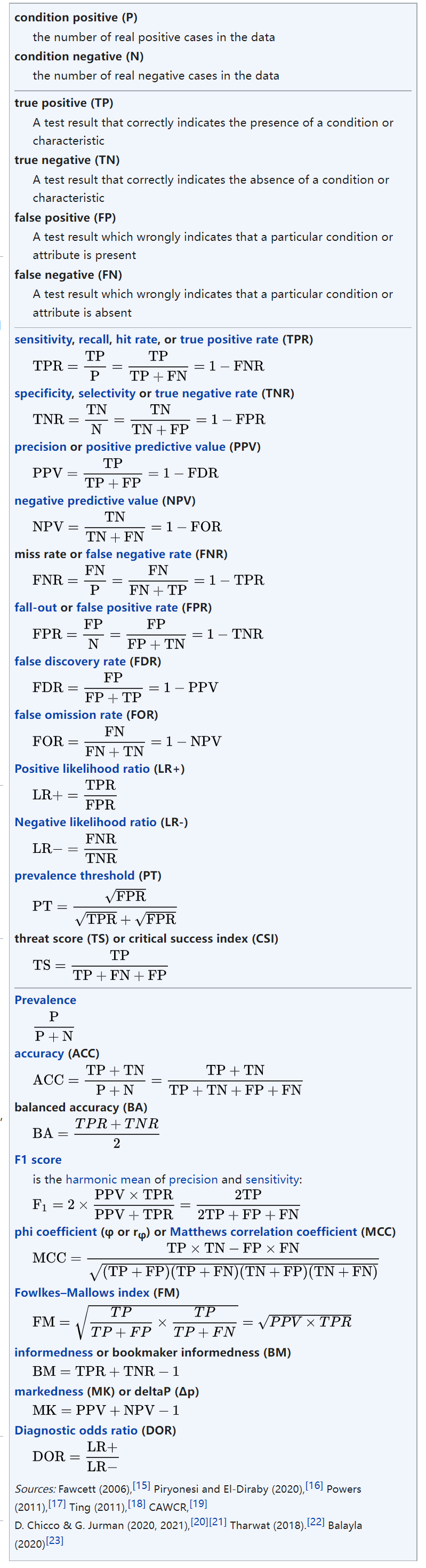
• Terminology and derivations from a confusion matrix

  

To plot the ROC curve, you first need to compute the TPR and FPR for various threshold values, using the roc_curve() function:

from sklearn.metrics import roc_curve
fpr, tpr, thresholds = roc_curve(y_train_5, y_scores)

def plot_roc_curve(fpr, tpr, label=None):
		plt.plot(fpr, tpr, linewidth=2, label=label)
		plt.plot([0, 1], [0, 1], 'k--') # dashed diagonal
		[...] # Add axis labels and grid
plot_roc_curve(fpr, tpr)
plt.show()

One way to compare classifiers is to measure the area under the curve (AUC). A perfect classifier will have a ROC AUC equal to 1, whereas a purely random classifier will have a ROC AUC equal to 0.5. Scikit-Learn provides a function to compute the ROC AUC:

As a rule of thumb, you should prefer the PR curve whenever the positive class is rare or when you care more about the false positives than the false negatives, and the ROC curve otherwise.

Let’s train a RandomForestClassifier and compare its ROC curve and ROC AUC
score to the SGDClassifier.

The RandomForestClassi fier class does not have a decision_function() method. Instead it has a pre dict_proba() method. Scikit-Learn classifiers generally have one or the other.

The predict_proba() method returns an array containing a row per instance and a column per class, each containing the probability that the given instance belongs to the given class.

from sklearn.ensemble import RandomForestClassifier
forest_clf = RandomForestClassifier(random_state=42)
y_probas_forest = cross_val_predict(forest_clf, X_train, y_train_5, cv=3,
																		method="predict_proba")
y_probas_forest

But to plot a ROC curve, you need scores, not probabilities. A simple solution is to
use the positive class’s probability as the score:

y_scores_forest = y_probas_forest[:, 1] # score = proba of positive class
fpr_forest, tpr_forest, thresholds_forest = roc_curve(y_train_5,y_scores_forest)

plt.plot(fpr, tpr, "b:", label="SGD")
plot_roc_curve(fpr_forest, tpr_forest, "Random Forest")
plt.legend(loc="lower right")
plt.show()

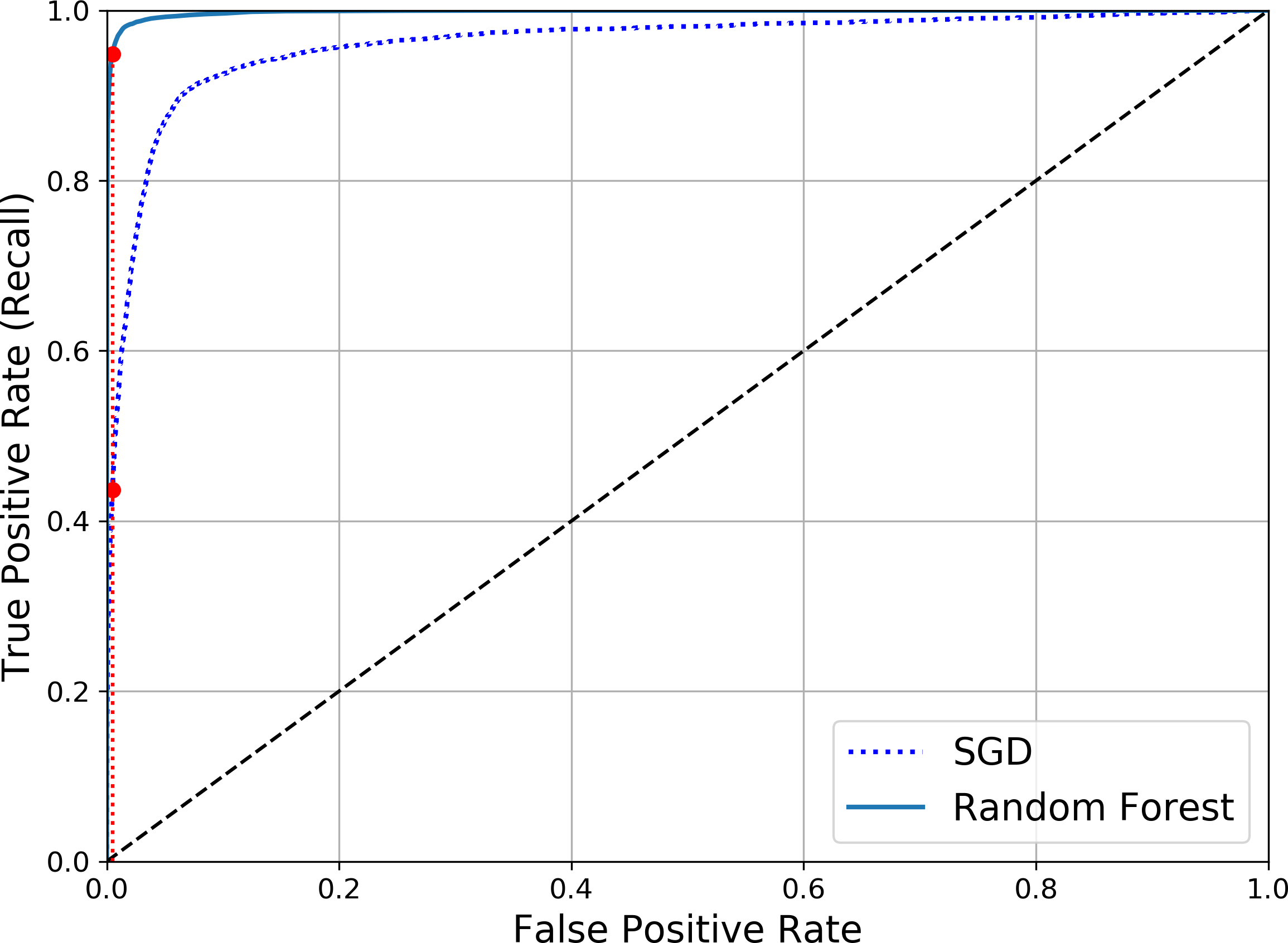
The RandomForestClassifier’s ROC curve looks much better than the SGDClassifier’s: it comes much closer to the top-left corner. As a result, its ROC AUC score is also significantly better:

>>> roc_auc_score(y_train_5, y_scores_forest)
0.9983436731328145

Multiclass Classification

• Some algorithms (such as Random Forest classifiers or naive Bayes classifiers) are
  capable of handling multiple classes directly.
• Others (such as Support Vector Machine classifiers or Linear classifiers) are strictly binary classifiers.
  • The one-versus-all (OvA) strategy
    • train 10 binary classifiers
  • The one-versus-one (OvO) strategy
    • training 45 binary classifiers
    • The main advantage of OvO is that each classifier only needs to be trained on the part of the training set for the two classes that it must distinguish.
  • Some algorithms (such as Support Vector Machine classifiers) scale poorly with the size of the training set, so for these algorithms OvO is preferred since it is faster to
    train many classifiers on small training sets than training few classifiers on large
    training sets. For most binary classification algorithms, however, OvA is preferred.

Scikit-Learn detects when you try to use a binary classification algorithm for a multiclass classification task, and it automatically runs OvA (except for SVM classifiers for which it uses OvO). Let’s try this with the SGDClassifier:

>>> sgd_clf.fit(X_train, y_train) # y_train, not y_train_5
>>> sgd_clf.predict([some_digit])
array([5], dtype=uint8)

Scikit-Learn actually trained 10 binary classifiers, got their decision scores for the
image, and selected the class with the highest score.

>>> some_digit_scores = sgd_clf.decision_function([some_digit])
>>> some_digit_scores
array([[-15955.22627845, -38080.96296175, -13326.66694897,
 573.52692379, -17680.6846644 , 2412.53175101,
 -25526.86498156, -12290.15704709, -7946.05205023,
 -10631.35888549]])

The highest score is indeed the one corresponding to class 5:

>>> np.argmax(some_digit_scores)
5
>>> sgd_clf.classes_
array([0, 1, 2, 3, 4, 5, 6, 7, 8, 9], dtype=uint8)
>>> sgd_clf.classes_[5]
5

When a classifier is trained, it stores the list of target classes in its classes_ attribute, ordered by value. In this case, the index of each class in the classes_ array conveniently matches the class itself (e.g., the class at index 5 happens to be class 5), but in general you won’t be so lucky.

Error Analysis

Here, we will assume that you have found a promising model and you want to find ways to improve it. One way to do this is to analyze the types of errors it makes.

First, you can look at the confusion matrix.

>>> y_train_pred = cross_val_predict(sgd_clf, X_train, y_train, cv=3)
>>> conf_mx = confusion_matrix(y_train, y_train_pred)
>>> conf_mx
array([[5578, 0, 22, 7, 8, 45, 35, 5, 222, 1],
 [ 0, 6410, 35, 26, 4, 44, 4, 8, 198, 13],
 [ 28, 27, 5232, 100, 74, 27, 68, 37, 354, 11],
 [ 23, 18, 115, 5254, 2, 209, 26, 38, 373, 73],
 [ 11, 14, 45, 12, 5219, 11, 33, 26, 299, 172],
 [ 26, 16, 31, 173, 54, 4484, 76, 14, 482, 65],
 [ 31, 17, 45, 2, 42, 98, 5556, 3, 123, 1],
 [ 20, 10, 53, 27, 50, 13, 3, 5696, 173, 220],
 [ 17, 64, 47, 91, 3, 125, 24, 11, 5421, 48],
 [ 24, 18, 29, 67, 116, 39, 1, 174, 329, 5152]])

That’s a lot of numbers. It’s often more convenient to look at an image representation
of the confusion matrix, using Matplotlib’s matshow() function:

plt.matshow(conf_mx, cmap=plt.cm.gray)
plt.show()

This confusion matrix looks fairly good, since most images are on the main diagonal, which means that they were classified correctly.

Compare error rates instead of absolute number of errors.

row_sums = conf_mx.sum(axis=1, keepdims=True)
norm_conf_mx = conf_mx / row_sums

np.fill_diagonal(norm_conf_mx, 0)
plt.matshow(norm_conf_mx, cmap=plt.cm.gray)
plt.show()

Now you can clearly see the kinds of errors the classifier makes. Remember that rows represent actual classes, while columns represent predicted classes. The column for class 8 is quite bright, which tells you that many images get misclassified as 8s.