


Series作为Dataframe的重要组成部分,Seires类似于一种带有索引的数组.
1.Series创建
创建Series出现报错:TypeError: Index(...) must be called with a collection of some kind, 'ABCD' was passed(索引(…)必须使用某种集合调用,也就是说索引必须是某种集合,我传递的却是字符串“ABCD”)
s1 = pd.Series(
    np.random.randint(10,20,size=4),
    index="ABCD",
    dtype="float64",
    name="age"
)
print(s1)
所以将index转换为list,tuple都是可以的
s1=pd.Series(
    np.random.randint(10,20,size=4),
    index=list("ABCD"),
    dtype="float64",
    name="age"
)
2.Series索引取值
存在位置索引和标签索引.方式如其名类似于list,用 index和标签而已,只是多了两种方法series.iloc[index],series.loc[label](integer location)
s1 = pd.Series(np.random.randint(10,20,size=4),index=list("ABCD"),dtype="float64",name="age")
print("S1>>\n",s1)
print("手动分割线".center(100,"-"))
print(s1[0])
print(s1.iloc[0])
print(s1["A"])
print(s1.loc["A"])
结果图: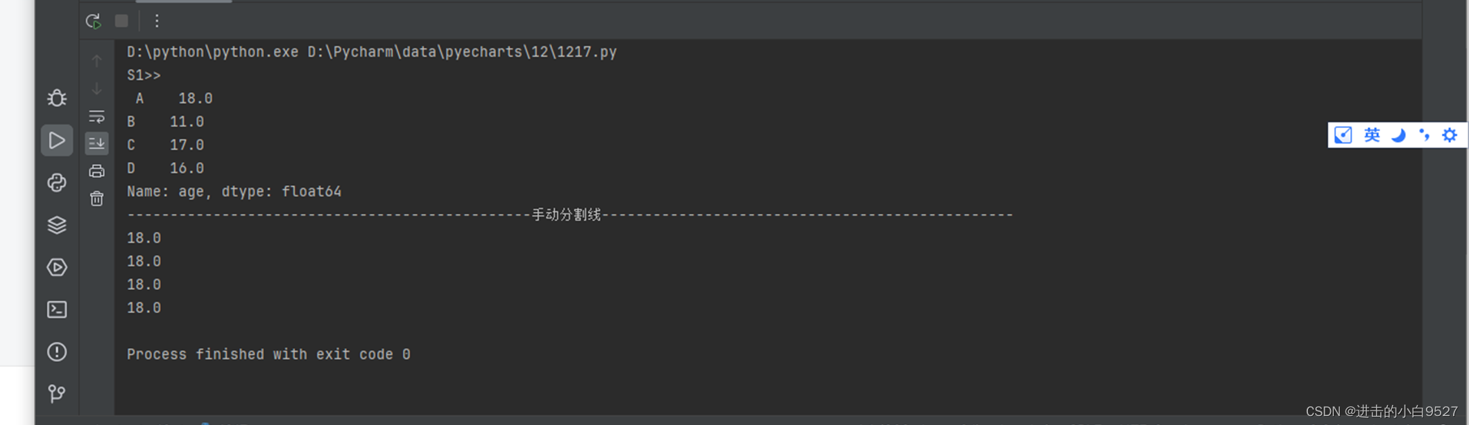
3.Series切片
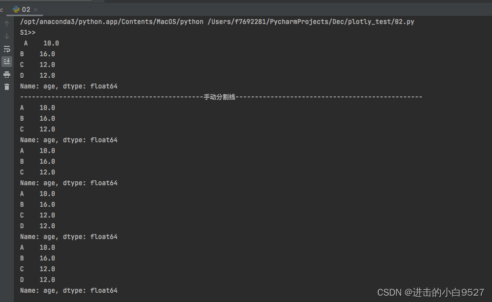
series的切片和列表的切片并无明显的不同,基于位置索引的切片(顾前不顾后),基于标签索引 的切片(顾前也顾后)
s1 = pd.Series(
    np.random.randint(10,20,size=4),
    index=list("ABCD"),
    dtype="float64",
    name="age"
)
print("S1>>\n",s1)
print("手动分割线".center(100,"-"))
print(s1[0:3])
print(s1.iloc[0:3])
print(s1["A":"D"])
print(s1.loc["A":"D"])
结果图:
4.Series属性
属性包括value,index,name,dtype,size,shape......
s1 = pd.Series(
    np.random.randint(10, 20, size=4),
    index=list("ABCD"),
    dtype="float64",
    name="age"
)
print("s1>>\n",s1)
print("手动分割线".center(100, "-"))
# series中数据值组成的numpy数组,都可以通过list()转化为list
print(s1.values, type(s1.values))
print(list(s1.values))
print("手动分割线".center(100, "-"))
# series索引组成的数组
print(s1.index, type(s1.index))
print(list(s1.index))
print("手动分割线".center(100, "-"))
# series的名字
print(s1.name, type(s1.name))
print("手动分割线".center(100, "-"))
# series的数据类型
print(s1.dtype)
print("手动分割线".center(100, "-"))
# series的维度,一维
print(s1.shape)
print("手动分割线".center(100, "-"))
# series中的元素个数
print(s1.size)
结果图:

5.将Series转化为DataFrame
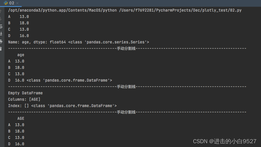
DataFrame作为pandas另外一种重要的数据结构,将series转化为DataFrame有大概两种实现方式。df1 = pd.DataFrame(s1),df3 = s1.to_frame(name="AGE")。
series指定的name会成为DataFrame结构的columns,clounms的类型也是集合类型,不能是单独的str.
使用 df2 = pd.DataFrame(s1,columns=["AGE"]),若series的name不存在则会生成为columns.若存在且发生冲突,则会变为Empty DataFrame。
使用df3 = s1.to_frame(name="AGE"),即使name名称发生冲突时也会被修改。
s1 = pd.Series(
    np.random.randint(10, 20, size=4),
    index=list("ABCD"),
    dtype="float64",
    name="age"
)
df1 = pd.DataFrame(s1)
print(s1,type(s1))
print("手动分割线".center(100,"-"))
print(df1,type(df1))
print("手动分割线".center(100,"-"))
df2 = pd.DataFrame(s1,columns=["AGE"])
print(df2,type(df2))
print("手动分割线".center(100,"-"))
df3 = s1.to_frame(name="AGE")
print(df3)
结果图:
DataFrame作为类二维数组,存在行和列,对应Excel的行和列标签
1.Dataframe的创建
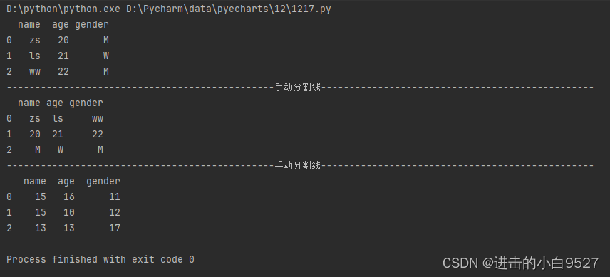
Datafrme的创建可以通过以下三种方式:
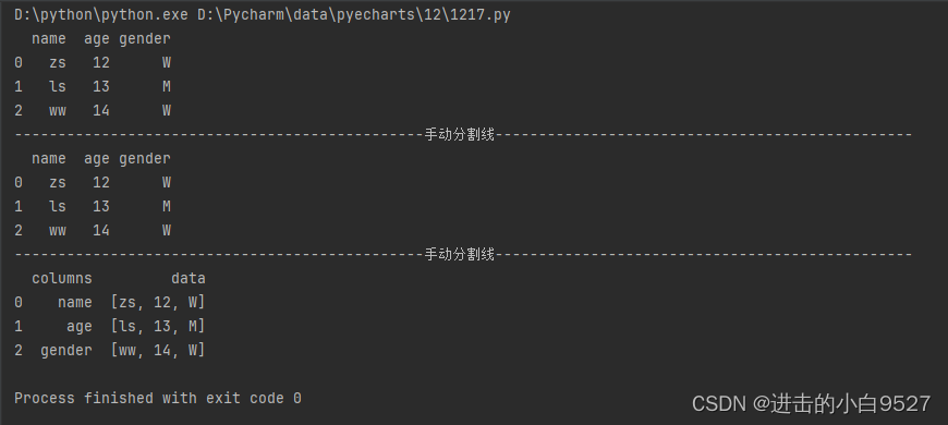
1.通过字典创建,字典的key作为columns,字典的value作为数据,插入的时候是按列进行插入的
2.通过列表嵌套列表,或是列表嵌套元祖,此时插入的列表是按行进行插入的
3.通过numpy数组创建Dataframe
data = {
    "name":["zs","ls","ww"],
    "age":[20,21,22],
    "gender":["M","W","M"]
}
df1 = pd.DataFrame(data)
print(df1)
print("手动分割线".center(100,"-"))
data2 = [
    ["zs","ls","ww"],
    [20,21,22],
    ["M","W","M"]
]
df2 = pd.DataFrame(data2,columns=("name","age","gender"))
print(df2)
print("手动分割线".center(100,"-"))
data3 = np.random.randint(10,20,size=(3,3))
df3 = pd.DataFrame(data3,columns=("name","age","gender"))
print(df3)
结果图:
2. Pandas实现文件的读取和写入
1.文件 读取包括各种类型文件的读取pd.read_excel(),pd.read_csv(),pd.read_json()
2.文件写入,包括df.to_excel,df.to_csv(),df.to_json(),写入文件时,index=False表示不会将默认的index进行写入.
3.读取CSV但是使用pd.read_excel()方法时会报错ValueError: Excel file format cannot be determined, you must specify an engine manually.(ValueError:无法确定Excel文件格式,必须手动指定引擎。

df1 = pd.DataFrame({
    "name": ["zs", "ls", "ww"],
    "age": [12, 13, 14],
    "gender": ["W", "M", "W"]
})
df1.to_excel("df1.xlsx", index=False)
df1_1 = pd.read_excel("./df1.xlsx")
print(df1_1)
print("手动分割线".center(100,"-"))

df2 = pd.DataFrame({
    "name": ["zs", "ls", "ww"],
    "age": [12, 13, 14],
    "gender": ["W", "M", "W"]
})
df2.to_csv("df2.csv",index=False)
df2_1 = pd.read_csv("./df2.csv")
print(df2_1)
print("手动分割线".center(100,"-"))

df3 = pd.DataFrame({
    "name": ["zs", "ls", "ww"],
    "age": [12, 13, 14],
    "gender": ["W", "M", "W"]
})
df3.to_json("df3.json", index=False, orient="split")
df3_1 = pd.read_json("./df3.json")
print(df3_1)
结果图:
3.Pandas实现Excel的多个sheet写入
Pandas的ExcelWriter对象支持将多个dataframe对象,写入到不同的sheet里面去
data1 = pd.DataFrame({"name":["zs","ls","ww"],"age":[12,13,14]})
data2 = pd.DataFrame(np.random.randint(10,20,size=(3,2)),columns=["name","age"])

with pd.ExcelWriter("./combine.xlsx",engine="openpyxl") as ew:
    data1.to_excel(ew,sheet_name="sheet_name1",index=False)
    data2.to_excel(ew,sheet_name="sheet_name2",index=False)
4.Pandas实现多层索引
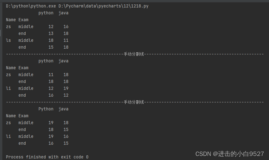
多层索引的实现,就是创建多个索引组,然后将索引给予对应的命名.再正常创建Datafram将多层索引赋值给index即可,常见的多层索引的创建有三种:
1.通过tuple创建多层索引,一对一的关系.
label_index = [("zs","middle"),("zs","end"),("ls","middle"),("ls","end")]
mult_index = pd.MultiIndex.from_tuples(label_index,names=["Name","Exam"])
2.通过Array进行创建,两个数组之间相应的元素一一对应.
label_index_2 = [["zs","zs","li","li"],["middle","end","middle","end"]]
mult_index_2 = pd.MultiIndex.from_arrays(label_index_2,names=["Name","Exam"])
3.创建多层索引的笛卡尔积,数组中的元素是相乘的关系,多个对多个
label_index_3 = [["zs","li"],["middle","end"]]
mult_index_3 = pd.MultiIndex.from_product(label_index_3,names=["Name","Exam"])
label_index = [("zs","middle"),("zs","end"),("ls","middle"),("ls","end")]
mult_index = pd.MultiIndex.from_tuples(label_index,names=["Name","Exam"])
df1 = pd.DataFrame(np.random.randint(10,20,size=(4,2)),index=mult_index,columns=["python","java"])
print(df1)
df1.to_excel("./mult.xlsx",sheet_name="df1")
print("手动分割线".center(100,"-"))
label_index_2 = [["zs","zs","li","li"],["middle","end","middle","end"]]
mult_index_2 = pd.MultiIndex.from_arrays(label_index_2,names=["Name","Exam"])
df2 = pd.DataFrame(np.random.randint(10,20,size=(4,2)),index=mult_index_2,columns=["python","java"])
print(df2)
print("手动分割线".center(100,"-"))
label_index_3 = [["zs","li"],["middle","end"]]
mult_index_3 = pd.MultiIndex.from_product(label_index_3,names=["Name","Exam"])
df3 = pd.DataFrame(np.random.randint(10,20,size=(4,2)),index=mult_index_3,columns=["Python","java"])
print(df3)
with pd.ExcelWriter("./mult.xlsx",engine="openpyxl") as ew:
df1.to_excel(ew,sheet_name="df1")
df2.to_excel(ew,sheet_name="df2")
df3.to_excel(ew,"df3")结果图:

5.Pandas多层索引的读写
多层索引读取主要是和index_col属性有关,此表示读取出来的内容的index,可以设置str也可以设置list,list里面可以是标签也可以是index下标。但是在使用list标签进行读取excel的时候出现报错,读取CSV的时候却没有问题......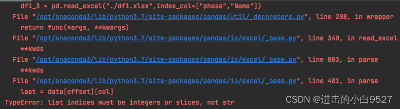
1.设置index_col不设置时,多层索引的合并单元格效果就会失去
import numpy as np
import pandas as pd

df1 = pd.DataFrame(
    np.random.randint(10,20,size=(6,2)),
    index=pd.MultiIndex.from_product([["ls","wu","zl"],["start","middle"]],names=["Name","phase"]),
    columns=["Python","Java"]
)
df1.to_csv("./df1.csv")
df1_0 = pd.read_csv("./df1.csv")
print(df1_0)
print("手动分割线".center(100,"-"))
df1_1 = pd.read_csv("./df1.csv",index_col=["Name","phase"])
print(df1_1)
效果图: 
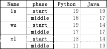
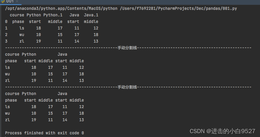
2.多层索引也可设置columns,但是会发现 to_excel()只要涉及多级表头,就会存在表头和内容之间存在空行,但是在CSV里面不存在此问题,但是CSV由于格式的问题,存入的合并单元各都是无效的。由此读取出来的内容也是有问题的,可以通过设置header,和index_col来设置行索引和列索引。
df2 = pd.DataFrame(
    np.random.randint(10, 20, size=(3, 4)),
    index=["ls", "wu", "zl"],
    columns=pd.MultiIndex.from_product([["Python", "Java"], ["start", "middle"]], names=["course", "phase"])
)
df2.to_csv("./df2.csv")
df2.to_excel("./df2.xlsx")
# 存入之后不设置header和index_col
df2_00 = pd.read_csv("./df2.csv")
print(df2_00)
print("手动分割线".center(100, "-"))
# 存入之后设置header和index_col
df2_0 = pd.read_csv("./df2.csv", header=[0, 1], index_col=0)
print(df2_0)
print("手动分割线".center(100, "-"))
# 读取excel
df2_1 = pd.read_excel("./df2.xlsx", header=[0, 1], index_col=0)
print(df2_1)
结果图:
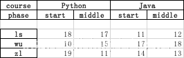
3.对于多层索引出现的表头和内容之间的空行问题:pandas中df的列索引和行索引都可以有name属性(多层索引就是names属性),所以一旦涉及多层索引,pandas需要预留位置来展示多层索引可能存在的names属性
找了很多方式无论是重设索引
df2 = df2.T.reset_index(level=1).T
还是删除空行,实现出来的都不是需要的效果
df2.dropna(inplace=True)
github上面给出的workaround是:
with pd.ExcelWriter("./df2.xlsx",engine="xlsxwriter") as ew:
    df2.to_excel(ew, sheet_name="test1")
    ew.sheets["test1"].set_row(2, None, None, {"hidden": True})
效果图:

6.数据重塑
1.数据重塑包括数据的转置(行列转化)
2.宽表的转化,df1.melt(),id_var指定为锚,保持不变,var_name指定之前作为表头的数据的name,value_name指定之前是数据的name.
def melt(
self,
id_vars=None,
value_vars=None,
var_name=None,
value_name="value",
col_level: Level | None = None,
ignore_index: bool = True,
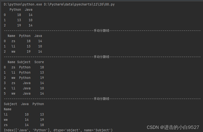
) -> DataFrame:3.长表的转化,df1.pivot(),index指定变化之后的索引名,coulmns指定变化之后的表头名里面包含的是表头的内容,value则是数据名称
def pivot(self, index=None, columns=None, values=None) -> DataFrame:import pandas as pd
import numpy as np
df1 = pd.DataFrame(
np.random.randint(10,20,size=(3,2)),
columns=["Python","Java"]
)
print(df1)
print("手动分割线".center(100,"-"))
df1.insert(loc=0,column="Name",value=["zs","li","ww"])
print(df1)
print("手动分割线".center(100,"-"))
df1_melt = df1.melt(id_vars="Name",var_name="Subject",value_name="Score")
print(df1_melt)
print("手动分割线".center(100,"-"))
df1_pivot = df1_melt.pivot(index="Name",columns="Subject",values="Score")
print(df1_pivot)
print(df1_pivot.columns)
print(df1_pivot.index)
df1_pivot.to_excel("df1_pivot.xlsx")结果图:
通过df.pivot()转化而来的数据,columns的标签名并不会写入excel,Name则会被写入,所以不会导致表头错位.

7.数据合并
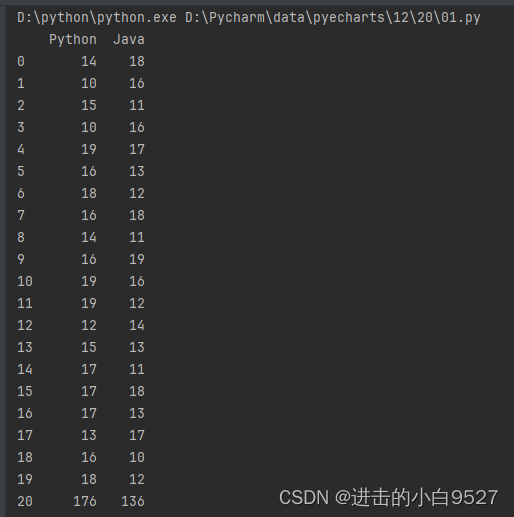
数据合并采用pd.concat()方法:,objs为数据对象,axis为合并的方向,默认方向为0为index方向,1为columns方向
def concat(
objs: Iterable[NDFrame] | Mapping[Hashable, NDFrame],
axis: Axis = 0,
join: str = "outer",
ignore_index: bool = False,
keys=None,
levels=None,
names=None,
verify_integrity: bool = False,
sort: bool = False,
copy: bool = True,
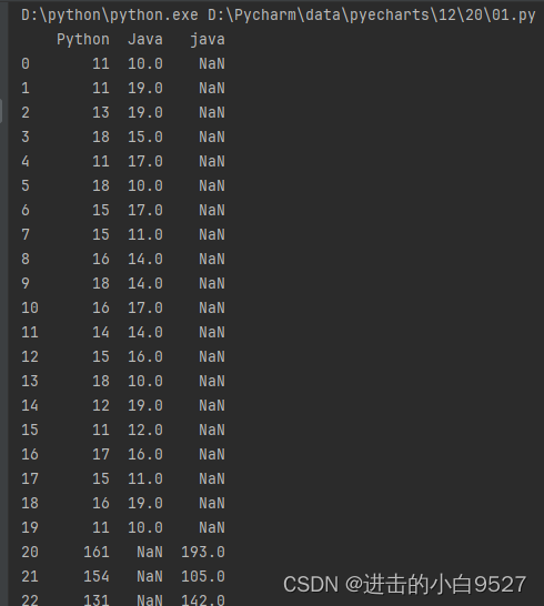
) -> DataFrame | Series:1.在index方向上面合并时,数据的columns的名字得是一样的,不然合并不同的列名时,产生的新的列用Nan进行补充
2.在columns方向上面合并时,数据的行不一样时,合并时缺少的数据用NaN补全
3.但是合并之后的index并不会改变需要使用reset_index()来将index重置,drop表示删除旧的index,inplace表示在本身进行修改.
def reset_index(
        self,
        level: Hashable | Sequence[Hashable] | None = None,
        drop: bool = False,
        inplace: bool = False,
        col_level: Hashable = 0,
        col_fill: Hashable = "",
    ) -> DataFrame | None:
import pandas as pd
import numpy as np
df1 = pd.DataFrame(
np.random.randint(10,20,size=(20,2)),
columns=["Python","Java"]
)
df2 = pd.DataFrame(
np.random.randint(100,200,size=(15,2)),
columns=["Python","Java"]
)
df_1_2 = pd.concat([df1,df2])
df_1_2.reset_index(drop=True,inplace=True)
print(df_1_2)结果图:
列名不一致时:
df1 = pd.DataFrame(
    np.random.randint(10,20,size=(20,2)),
    columns=["Python","Java"]
)
df2 = pd.DataFrame(
    np.random.randint(100,200,size=(15,2)),
    columns=["Python","java"]
)
df_1_2 = pd.concat([df1,df2])
df_1_2.reset_index(drop=True,inplace=True)
print(df_1_2)
结果图:
8.数据融合
pd.merge()基于列的合并操作,将两个Dataframe基于共同的列进行融合
1.on为融合的锚点
2.how为融合的方式 how : {'left', 'right', 'outer', 'inner'},左,右,全部,相同
def merge(
    left: DataFrame | Series,
    right: DataFrame | Series,
    how: str = "inner",
    on: IndexLabel | None = None,
    left_on: IndexLabel | None = None,
    right_on: IndexLabel | None = None,
    left_index: bool = False,
    right_index: bool = False,
    sort: bool = False,
    suffixes: Suffixes = ("_x", "_y"),
    copy: bool = True,
    indicator: bool = False,
    validate: str | None = None,
) -> DataFrame:
import pandas as pd
import numpy as np
df1 = pd.DataFrame({
"ID": [1, 2, 3],
"Name": ["zs", "ls", "ww"]
})
df2 = pd.DataFrame({
"ID": [2, 3, 4],
"Age": [20, 21, 22]
})
df3 = pd.DataFrame(
{
"id": [2, 3, 4],
"Age": [20, 21, 22]
}
)
# 基于ID进行融合,显示ID相同的数据
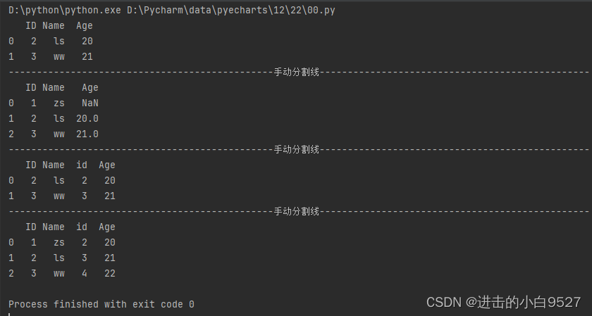
df_m = pd.merge(df1, df2, on="ID")
print(df_m)
print("手动分割线".center(100, "-"))
# 基于左边的ID进行融合,左边的ID内容保持不变,右边缺少的用NaN补充
df_m2 = pd.merge(df1, df2, on="ID", how="left")
print(df_m2)
print("手动分割线".center(100, "-"))
# 当融合时,两个Dataframe的列索引不一样时,会报错,此时可以用左右两个索引
# df_m3 = pd.merge(df1, df3, how="left")
df_m3 = pd.merge(df1, df3, left_on="ID", right_on="id")
print(df_m3)
print("手动分割线".center(100, "-"))
df_c4 = pd.concat([df1,df3],axis=1)
print(df_c4)结果图:
import pandas as pd
import numpy as np
df = pd.DataFrame(np.random.randint(10, 20, size=(5, 2)), columns=["Python", "Java"])
# 1.基于数据融合
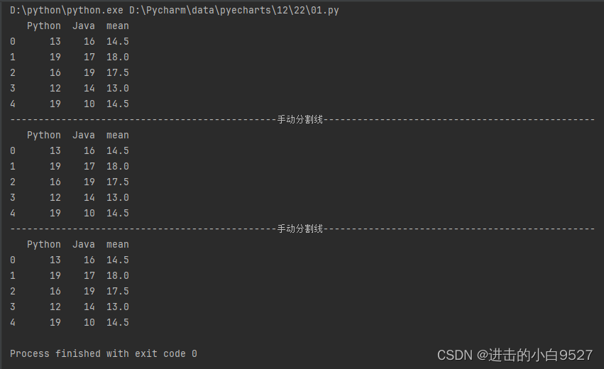
df1 = df.mean(axis=1).to_frame(name="mean")
df_m = pd.merge(df, df1, left_index=True, right_index=True)
print(df_m)
print("手动分割线".center(100, "-"))
# 2.基于数据合并
df_c = pd.concat([df, df1], axis=1)
print(df_c)
print("手动分割线".center(100, "-"))
# 3.基于数据列的添加
df["mean"] = np.mean(df, axis=1)
print(df)结果图:
9.数据连接
df1.join(df2),通过共同的索引或是共同的列将两个Dataframe的数据进行融合,感觉和数据融合没什么不同.只不过要保证共同的索引和共同的列有重叠的部分.
# how : {'left', 'right', 'outer', 'inner'}, default 'left'
def join(
        self,
        other: DataFrame | Series,
        on: IndexLabel | None = None,
        how: str = "left",
        lsuffix: str = "",
        rsuffix: str = "",
        sort: bool = False,
    ) -> DataFrame:
import pandas as pd
import numpy as np
df_employ = pd.DataFrame(
{"Num":[101,102,103,104],"Name":["zs","li","ww","zl"],"part":["HR","market","engineering","code"]}
)
df_salary = pd.DataFrame(
{
"Num":[102,103,104,105],
"salary":[10000,15000,12000,19000]
}
)
df_j = df_employ.set_index("Num").join(df_salary.set_index("Num"),how="inner")
print(df_j)
print("手动分割线".center(100,"-"))
df_m = pd.merge(df_employ,df_salary).set_index("Num")
print(df_m)结果图:

重设索引:df.set_index()
 """
        Set the DataFrame index using existing columns.

        Set the DataFrame index (row labels) using one or more existing
        columns or arrays (of the correct length). The index can replace the
        existing index or expand on it.
"""
def set_index(
        self,
        keys,
        drop: bool = True,
        append: bool = False,
        inplace: bool = False,
        verify_integrity: bool = False,
    ):
10.数据筛选
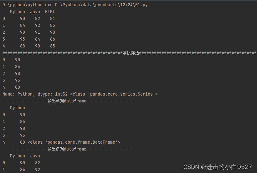
10.1通过字段也就是列名筛选数据
筛选出来的数据可以是个series也可以是个Dataframe.
import pandas as pd
import numpy as np

df = pd.DataFrame(
    data=np.random.randint(80, 100, size=(5, 3)),
    columns=["Python", "Java", "HTML"]
)
print(df)
print("字段筛选".center(100, "*"))
# 输出Series
print(df["Python"], type(df["Python"]))
# 输出单列dataframe
print("输出单列dataframe".center(50, "-"))
print(df[["Python"]], type(df[["Python"]]))
# 输出多列dataframe
print("输出多列dataframe".center(50, "-"))
print(df[["Python","Java"]], type(df[["Python","Java"]]))
结果图:
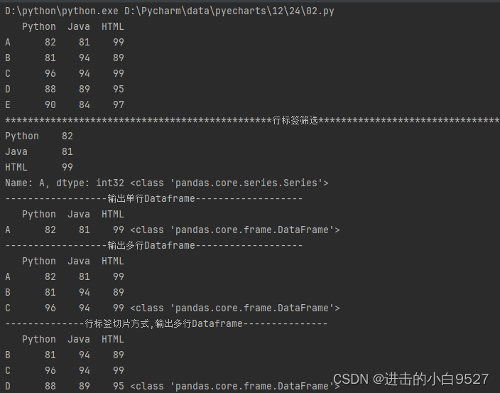
 10.2 行标签进行数据筛选
行标签筛选数据df.loc()选取数据行,可选取series和Dataframe,并可以通过指定行列来获取指定的元素
import pandas as pd
import numpy as np
df = pd.DataFrame(
data=np.random.randint(80, 100, size=(5, 3)),
columns=["Python", "Java", "HTML"],
index=["A","B","C","D","E"]
)
print(df)
# 输出series
print("行标签筛选".center(100,"*"))
print(df.loc["A"],type(df.loc["A"]))
# 输出单行Dataframe
print("输出单行Dataframe".center(50,"-"))
print(df.loc[["A"]],type(df.loc[["A"]]))
# 输出多行Dataframe
print("输出多行Dataframe".center(50,"-"))
print(df.loc[["A","B","C"]],type(df.loc[["A","B","C"]]))
# 行标签切片方式,输出多行Dataframe
print("行标签切片方式,输出多行Dataframe".center(50,"-"))
print(df.loc["B":"D"],type(df.loc["B":"D"]))
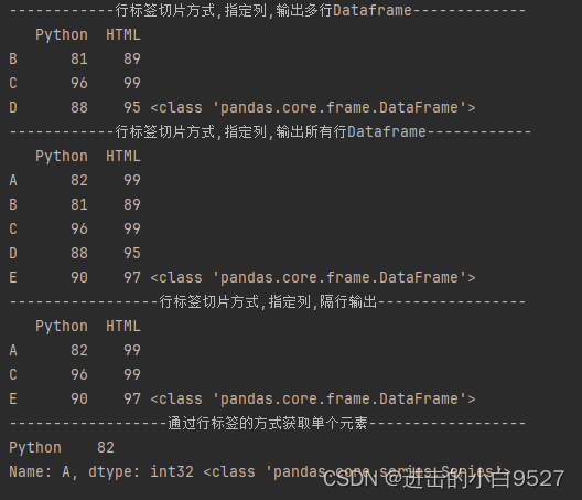
# 行标签切片方式,指定列,输出多行Dataframe
print("行标签切片方式,指定列,输出多行Dataframe".center(50,"-"))
print(df.loc["B":"D",["Python","HTML"]],type(df.loc["B":"D",["Python","HTML"]]))
# 行标签切片方式,指定列,输出所有行Dataframe
print("行标签切片方式,指定列,输出所有行Dataframe".center(50,"-"))
print(df.loc[:,["Python","HTML"]],type(df.loc[:,["Python","HTML"]]))
# 行标签切片方式,指定列,隔行输出
print("行标签切片方式,指定列,隔行输出".center(50,"-"))
print(df.loc[::2,["Python","HTML"]],type(df.loc[::2,["Python","HTML"]]))
# 通过行标签的方式获取单个元素
print("通过行标签的方式获取单个元素".center(50,"-"))
print(df.loc["A",["Python"]],type(df.loc["A",["Python"]]))结果图:
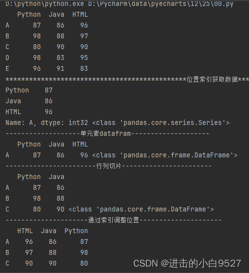
10.3 通过位置索引进行数据筛选
本质和标签筛选并无不同,只是使用的方法是df.iloc(),可以使用行列切片,也可以通过调整索引来调整行列中的位置关系
import pandas as pd
import numpy as np

df = pd.DataFrame(
    np.random.randint(80,100,size=(5,3)),
    columns=["Python","Java","HTML"],
    index=["A","B","C","D","E"]
)
print(df)
print("位置索引获取数据".center(100,"*"))
print(df.iloc[0],type(df.iloc[0]))
print("单元素datafram".center(50,"-"))
print(df.iloc[[0]],type(df.iloc[[0]]))
print("行列切片".center(50,"-"))
print(df.iloc[0:3,0:2],type(df.iloc[0:3,0:2]))
print("通过索引调整位置".center(50,"-"))
print(df.iloc[0:3,[2,1,0]])
结果图:
10.4 通过布尔索引进行数据筛选
布尔索引也可以被称为索引掩码,可以通过布尔运算来得到一组True和False的Series或是Dataframe,通过原有数组的掩码操作,将为True的值取出来.可以使用比较运算符(>,<,>=,<=,!=)或是逻辑运算符(&,|,~),使用& | ~时,生成的布尔列表外面得加上()
import pandas as pd
import numpy as np

df = pd.DataFrame(
    np.random.randint(0, 101, size=(8, 3)),
    columns=["Python", "Java", "HTML"]
)
print(df)
print("布尔索引获取数据".center(100, "*"))
print(df["Python"] > 50, type(df["Python"] > 30))
print(df[df["Python"] > 50])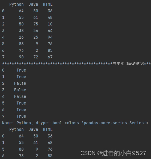
支持多条件筛选
print("支持& | ~实现多条件筛选".center(50, "-"))
print((df["Python"] > 50) & (df["HTML"] < 40))
print(df[(df["Python"] > 50) & (df["HTML"] < 40)])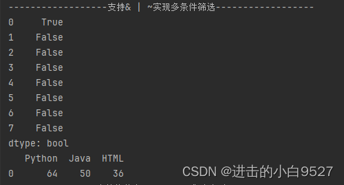
支持将整个dataframe作为索引',空值会被填充为NaN
print("支持将整个dataframe作为索引".center(50, "-"))
print(df>50,type(df>50))
print(df[df>50])
支持只筛选自己定义数组里面的数据
print("支持只筛选自己定义数组里面的数据".center(50, "-"))
print(df["Python"].isin([30,50,77]),type(df["Python"].isin([30,50,77])))
print(df[df["Python"].isin([30,50,77])])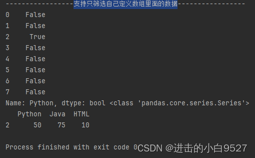
import pandas as pd
import numpy as np
df = pd.DataFrame(
np.random.randint(0, 101, size=(8, 3)),
columns=["Python", "Java", "HTML"]
)
print(df)
print("布尔索引获取数据".center(100, "*"))
print(df["Python"] > 50, type(df["Python"] > 30))
print(df[df["Python"] > 50])
print("支持& | ~实现多条件筛选".center(50, "-"))
print((df["Python"] > 50) & (df["HTML"] < 40))
print(df[(df["Python"] > 50) & (df["HTML"] < 40)])
print("支持将整个dataframe作为索引".center(50, "-"))
print(df>50,type(df>50))
print(df[df>50])
print("支持只筛选自己定义数组里面的数据".center(50, "-"))
print(df["Python"].isin([30,50,77]),type(df["Python"].isin([30,50,77])))
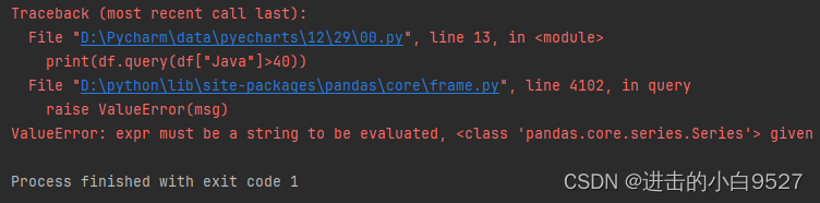
print(df[df["Python"].isin([30,50,77])])10.5 通过query进行查询
query里面的参数得是str类型,如果使用布尔索引就会报错 df.query(df["Java"] > 40)
ef query(self, expr: str, inplace: bool = False, **kwargs):
        """
        Query the columns of a DataFrame with a boolean expression.

        Parameters
        ----------
        expr : str
            The query string to evaluate.
        For example, if one of your columns is called ``a a`` and you want
            to sum it with ``b``, your query should be ```a a` + b``.
        Examples
        --------
        >>> df = pd.DataFrame({'A': range(1, 6),
        ...                    'B': range(10, 0, -2),
        ...                    'C C': range(10, 5, -1)})
        >>> df
           A   B  C C
        0  1  10   10
        1  2   8    9
        2  3   6    8
        3  4   4    7
        4  5   2    6
        >>> df.query('A > B')
           A  B  C C
        4  5  2    6

        The previous expression is equivalent to

        >>> df[df.A > df.B]
           A  B  C C
        4  5  2    6
import pandas as pd
import numpy as np
df = pd.DataFrame(
np.random.randint(10, 50, size=(5, 3)),
columns=["Java", "Python", "HTML"],
)
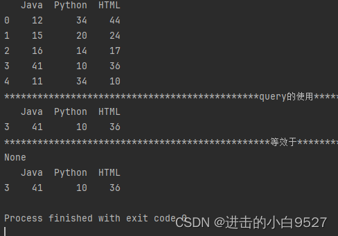
print(df)
print("query的使用".center(100, "*"))
print(df.query("Java > 40 and Python< 30"))
print(print("等效于".center(100, "*")))
print(df[(df["Java"]>40) & (df["Python"]<30)])结果图:
11.修改DataFrame数据
可以增加数据,修改数据的单个值,修改数据的多个值,修改数据的整列值,根据条件修改数据的值等
import pandas as pd
import numpy as np
df = pd.DataFrame(
data=np.random.randint(20, 30, size=(5, 3)),
columns=["Python", "Java", "HTML"],
index=list("ABCDE")
)
print("修改Dataframe的数据".center(100, "*"))
print(df)
print("插入Dataframe的数据".center(50, "-"))
df["PHP"] = pd.Series(np.random.randint(100, 200, size=5), index=list("ABCDE"))
print(df)
print("loc修改一个数据".center(50, "-"))
df.loc["A", "Python"] = 100
print(df)
print("iloc修改一个数据".center(50, "-"))
df.iloc[0, 1] = 200
print(df)
print("iloc修改多个数据".center(50, "-"))
df.iloc[0:1, 2:4] = 400
print(df)
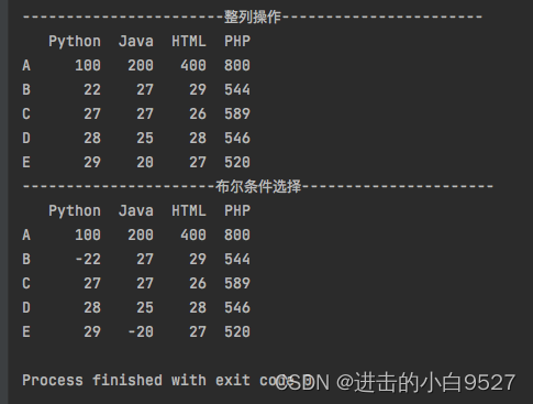
print("整列操作".center(50, "-"))
df["PHP"] += 400
print(df)
print("布尔条件选择".center(50, "-"))
df[df < 25] = -df
print(df)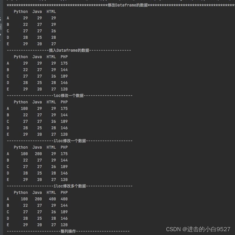
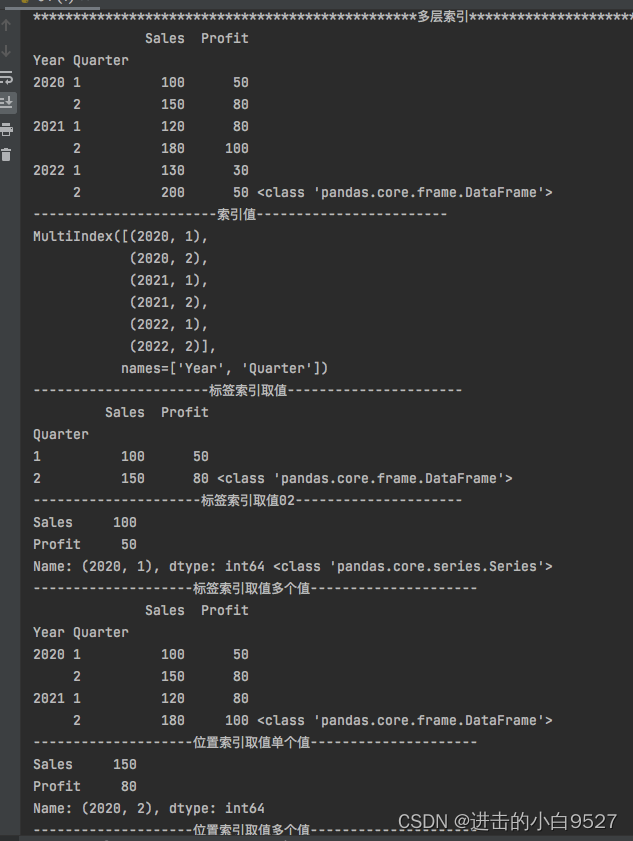
12.多层索引筛选数据
多层索引的取值和单个索引的取值并无不同,都是使用iloc()和loc()两种方式来实现。只是相对于标签索引取值而言,多了一个索引而已。而位置索引取值基本上没有变化。
import pandas as pd

data = {
    'Year': [2020, 2020, 2021, 2021, 2022, 2022],
    "Quarter": [1, 2, 1, 2, 1, 2],
    "Sales": [100, 150, 120, 180, 130, 200],
    "Profit": [50, 80, 80, 100, 30, 50]
}
df = pd.DataFrame(data)
df.set_index(["Year","Quarter"],inplace=True)
print("多层索引".center(100,"*"))
print(df,type(df))
print("索引值".center(50,"-"))
print(df.index)
print("标签索引取值".center(50,"-"))
print(df.loc[2020],type(df.loc[2020]))
print("标签索引取值02".center(50,"-"))
print(df.loc[(2020,1)],type(df.loc[(2020,1)]))
print("标签索引取值多个值".center(50,"-"))
print(df.loc[[2020,2021]],type(df.loc[[2020,2021]]))
print("位置索引取值单个值".center(50,"-"))
print(df.iloc[1])
print("位置索引取值多个值".center(50,"-"))
print(df.iloc[[0,1]])
效果图:
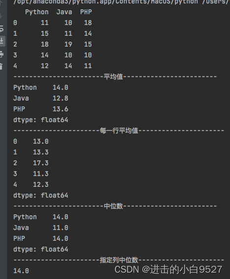
13.简单统计函数
可以使用df.mean()直接求平均值,使用df.mean(axix=1),指定方向为横向。使用简单的统计函数包括以下:
mean():平均值
median():中位数
sum():数据之和
min():数据最小值
max():数据最大值
std():计算数据的标准差
var():计算数据的方差
import pandas as pd
import numpy as np

df = pd.DataFrame(np.random.randint(10,20,size=(5,3)),columns=["Python","Java","PHP"])
print(df)
print("平均值".center(50,"-"))
print(df.mean())
print("每一行平均值".center(50,"-"))
print(df.mean(axis=1).round(1))
print("中位数".center(50,"-"))
print(df.median())
print("指定列中位数".center(50,"-"))
print(df["Python"].median())
效果图:
14.相关性分析函数
14.1 协方差
cov()计算协方差,协方差可以简单的反应两组统计样本的相关性,值为正,则表示正相关;值为负,则表示负相关。值为0,表示不相关,绝对值越大相关性越强。
def cov(self, min_periods=None):
"""
Compute pairwise covariance of columns, excluding NA/null values.

        Compute the pairwise covariance among the series of a DataFrame.
        The returned data frame is the `covariance matrix
Examples
        --------
        >>> df = pd.DataFrame([(1, 2), (0, 3), (2, 0), (1, 1)],
        ...                   columns=['dogs', 'cats'])
        >>> df.cov()
                  dogs      cats
        dogs  0.666667 -1.000000
        cats -1.000000  1.666667

        >>> np.random.seed(42)
        >>> df = pd.DataFrame(np.random.randn(1000, 5),
        ...                   columns=['a', 'b', 'c', 'd', 'e'])
        >>> df.cov()
                  a         b         c         d         e
        a  0.998438 -0.020161  0.059277 -0.008943  0.014144
        b -0.020161  1.059352 -0.008543 -0.024738  0.009826
        c  0.059277 -0.008543  1.010670 -0.001486 -0.000271
        d -0.008943 -0.024738 -0.001486  0.921297 -0.013692
        e  0.014144  0.009826 -0.000271 -0.013692  0.977795
"""
很明显使用df.cov()求出来的是四个 dogs&dogs,dogs&cats,cats&dogs,cats&cats之间的数值,而协方差的计算公式为:
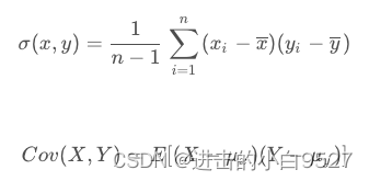
求均值->求离差->离差成绩之和/n-1
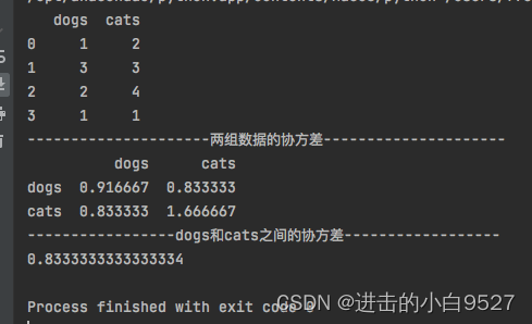
import pandas as pd
import numpy as np

df0 = pd.DataFrame([(1, 2), (3, 3), (2, 4), (1, 1)], columns=['dogs', 'cats'])
print(df0)
print("两组数据的协方差".center(50, "-"))
print(df0.cov())
# 均值
mean_dogs = np.mean(df0["dogs"])
mean_cats = np.mean(df0["cats"])
# # 离差
dev_dogs = df0["dogs"] - mean_dogs
dev_cats = df0["cats"] - mean_cats
# # 协方差
cov = sum(dev_dogs * dev_cats)/(len(dev_dogs)-1)
print("dogs和cats之间的协方差".center(50, "-"))
print(cov)
结果图:
14.2 相关性系数
corr()计算相关性系数。使用协方差比较两组数据的相关性时,如果数据中间存在极值,会影响两组数据之间的相关性,所以需要引入加权平均。python引入了相关系数来分析两组数据之间的相关性。相关性系数是介于【-1,1】之间的数字和协方差的表示的概念相类似。
pearson:皮尔逊相关系数,用于测量线性关系
kendall:肯德尔相关系数,用于测量有序分类变量之间的相关性
spearman:斯皮尔曼相关系数,用于测量有序分类变量之间的相关性
    def corr(self, method="pearson", min_periods=1):
        """
        Compute pairwise correlation of columns, excluding NA/null values.

        Parameters
        ----------
        method : {'pearson', 'kendall', 'spearman'} or callable
            * pearson : standard correlation coefficient
            * kendall : Kendall Tau correlation coefficient
            * spearman : Spearman rank correlation
            * callable: callable with input two 1d ndarrays
                and returning a float. Note that the returned matrix from corr
                will have 1 along the diagonals and will be symmetric
                regardless of the callable's behavior
                .. versionadded:: 0.24.0

        min_periods : int, optional
            Minimum number of observations required per pair of columns
            to have a valid result. Currently only available for Pearson
            and Spearman correlation.

        Returns
        -------
        DataFrame
            Correlation matrix.
“”“
df.corr()求解出来的结果和协方差类似,计算公式为
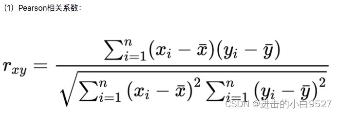
在求解出协方差的基础上->求标准差->协方差/标准差的乘积
求解标准差时存在,总体标准差(底数为n)和样本标准差(底数为n-1)
def std(a, axis=None, dtype=None, out=None, ddof=0, keepdims=np._NoValue):
    """
    Compute the standard deviation along the specified axis.

    Returns the standard deviation, a measure of the spread of a distribution,
    of the array elements. The standard deviation is computed for the
    flattened array by default, otherwise over the specified axis.

    Parameters
    ----------
    a : array_like
        Calculate the standard deviation of these values.
    axis : None or int or tuple of ints, optional
        Axis or axes along which the standard deviation is computed. The
        default is to compute the standard deviation of the flattened array.

        .. versionadded:: 1.7.0

        If this is a tuple of ints, a standard deviation is performed over
        multiple axes, instead of a single axis or all the axes as before.
    dtype : dtype, optional
        Type to use in computing the standard deviation. For arrays of
        integer type the default is float64, for arrays of float types it is
        the same as the array type.
    out : ndarray, optional
        Alternative output array in which to place the result. It must have
        the same shape as the expected output but the type (of the calculated
        values) will be cast if necessary.
    ddof : int, optional
        Means Delta Degrees of Freedom.  The divisor used in calculations
        is ``N - ddof``, where ``N`` represents the number of elements.
        By default `ddof` is zero.
"""
df0 = pd.DataFrame([(1, 2), (3, 3), (2, 4), (1, 1)], columns=['dogs', 'cats'])
print("总体标准差".center(50, "-"))
std_dogs = np.std(df0["dogs"])
print(std_dogs)
print("样本标准差".center(50, "-"))
std_dogs_dd = np.std(df0["dogs"], ddof=1)
print(std_dogs_dd)import pandas as pd
import numpy as np
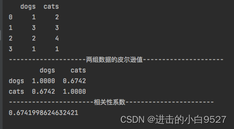
df0 = pd.DataFrame([(1, 2), (3, 3), (2, 4), (1, 1)], columns=['dogs', 'cats'])
print(df0)
print("两组数据的皮尔逊值".center(50, "-"))
print(df0.corr(method="pearson"))
# 均值
mean_dogs = np.mean(df0["dogs"])
mean_cats = np.mean(df0["cats"])
# 离差
dev_dogs = df0["dogs"] - mean_dogs
dev_cats = df0["cats"] - mean_cats
# 协方差
cov = sum(dev_dogs * dev_cats) / (len(dev_dogs)-1)
# 样本标准差
std_dogs = np.std(df0["dogs"], ddof=1)
std_ctas = np.std(df0["cats"], ddof=1)
# 相关性系数
corr = cov / (std_dogs * std_ctas)
print("相关性系数".center(50, "-"))
print(corr)结果图:
15.多层索引的分组聚合计算
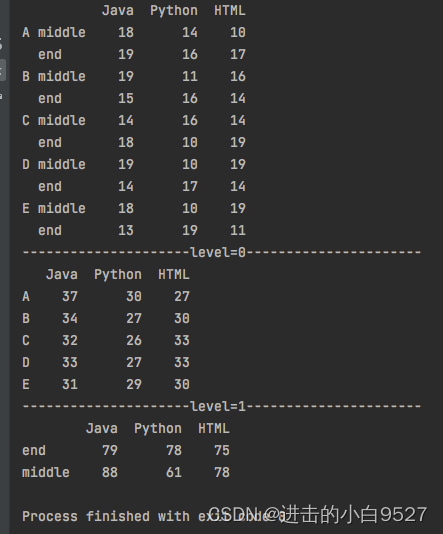
使用groupby()进行分组,在通过df.sum()等函数进行聚合运算,多层索引时可以通过指定参数level,进行不同组的聚合
“”“
We can groupby different levels of a hierarchical index
        using the `level` parameter:

        >>> arrays = [['Falcon', 'Falcon', 'Parrot', 'Parrot'],
        ...           ['Captive', 'Wild', 'Captive', 'Wild']]
        >>> index = pd.MultiIndex.from_arrays(arrays, names=('Animal', 'Type'))
        >>> df = pd.DataFrame({'Max Speed': [390., 350., 30., 20.]},
        ...                   index=index)
        >>> df
                        Max Speed
        Animal Type
        Falcon Captive      390.0
               Wild         350.0
        Parrot Captive       30.0
               Wild          20.0
        >>> df.groupby(level=0).mean()
                Max Speed
        Animal
        Falcon      370.0
        Parrot       25.0
        >>> df.groupby(level=1).mean()
                 Max Speed
        Type
        Captive      210.0
        Wild         185.0
        """
import pandas as pd
import numpy as np
df = pd.DataFrame(
np.random.randint(10,20,size=(10,3)),
columns=["Java","Python","HTML"],
index=pd.MultiIndex.from_product([list("ABCDE"),["middle","end"]])
)
print(df)
print("level=0".center(50,"-"))
a = df.groupby(level=0).sum()
print(a)
print("level=1".center(50,"-"))
a = df.groupby(level=1).sum()
print(a)结果图:
16.空数据的处理
16.1 空数据的删除
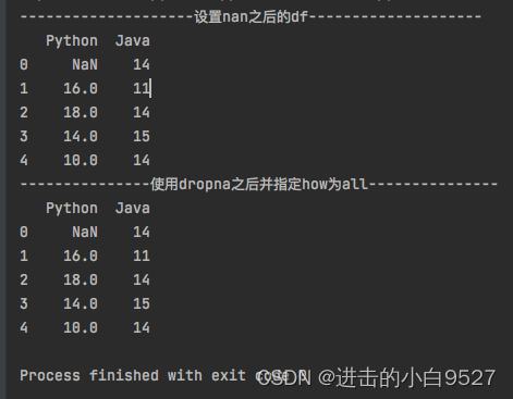
空数据的处理包括空数据的删除和填充,可以使用dropna()方法删除包含空数据(NaN)的行或是列。通过axis指定删除空值的行或是列,默认为行;how指定是一个值为空就删除还是所有值为空才删除。
 def dropna(self, axis=0, how="any", thresh=None, subset=None, inplace=False):
        """
        Remove missing values.

        See the :ref:`User Guide <missing_data>` for more on which values are
        considered missing, and how to work with missing data.

        Parameters
        ----------
        axis : {0 or 'index', 1 or 'columns'}, default 0
            Determine if rows or columns which contain missing values are
            removed.

            * 0, or 'index' : Drop rows which contain missing values.
            * 1, or 'columns' : Drop columns which contain missing value.

            .. deprecated:: 0.23.0

               Pass tuple or list to drop on multiple axes.
               Only a single axis is allowed.

        how : {'any', 'all'}, default 'any'
            Determine if row or column is removed from DataFrame, when we have
            at least one NA or all NA.

            * 'any' : If any NA values are present, drop that row or column.
            * 'all' : If all values are NA, drop that row or column.

        thresh : int, optional
            Require that many non-NA values.
        subset : array-like, optional
            Labels along other axis to consider, e.g. if you are dropping rows
            these would be a list of columns to include.
        inplace : bool, default False
            If True, do operation inplace and return None.

        Returns
        -------
        DataFrame
            DataFrame with NA entries dropped from it.
"""
import pandas as pd
import numpy as np
df = pd.DataFrame(
np.random.randint(10, 20, size=(5, 2)),
columns=["Python", "Java"]
)
df.iloc[0, 0] = np.nan
print("设置nan之后的df".center(50,"-"))
print(df)
print("使用dropna之后的df".center(50,"-"))
df.dropna(inplace=True)
print(df)
print("使用dropna之后指定列的df".center(50,"-"))
df.dropna(inplace=True,axis=1)
print(df)
print("使用dropna之后并指定how为all".center(50,"-"))
df.dropna(inplace=True,how="all")
print(df)
结果图:
16.2 空数据的填充
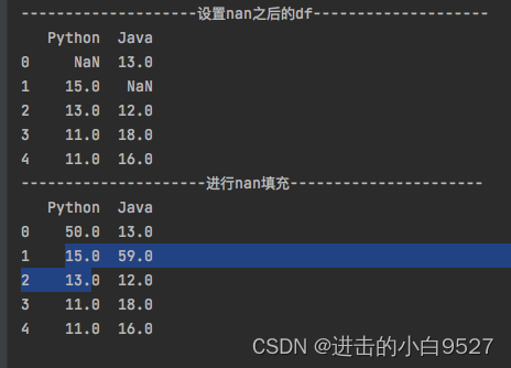
使用fillna()来填充数据中的空数据(NaN)
    def fillna(
        self,
        value=None,
        method=None,
        axis=None,
        inplace=False,
        limit=None,
        downcast=None,
    ):
        """
        Fill NA/NaN values using the specified method.

        Parameters
        ----------
        value : scalar, dict, Series, or DataFrame
            Value to use to fill holes (e.g. 0), alternately a
            dict/Series/DataFrame of values specifying which value to use for
            each index (for a Series) or column (for a DataFrame).  Values not
            in the dict/Series/DataFrame will not be filled. This value cannot
            be a list.
        method : {'backfill', 'bfill', 'pad', 'ffill', None}, default None
            Method to use for filling holes in reindexed Series
            pad / ffill: propagate last valid observation forward to next valid
            backfill / bfill: use next valid observation to fill gap.
        axis : %(axes_single_arg)s
            Axis along which to fill missing values.
        inplace : bool, default False
            If True, fill in-place. Note: this will modify any
            other views on this object (e.g., a no-copy slice for a column in a
            DataFrame).
        limit : int, default None
            If method is specified, this is the maximum number of consecutive
            NaN values to forward/backward fill. In other words, if there is
            a gap with more than this number of consecutive NaNs, it will only
            be partially filled. If method is not specified, this is the
            maximum number of entries along the entire axis where NaNs will be
            filled. Must be greater than 0 if not None.
        downcast : dict, default is None
            A dict of item->dtype of what to downcast if possible,
            or the string 'infer' which will try to downcast to an appropriate
            equal type (e.g. float64 to int64 if possible).

        Returns
        -------
        %(klass)s
            Object with missing values filled.

        See Also
        --------
        interpolate : Fill NaN values using interpolation.
        reindex : Conform object to new index.
        asfreq : Convert TimeSeries to specified frequency.

        Examples
        --------
        >>> df = pd.DataFrame([[np.nan, 2, np.nan, 0],
        ...                    [3, 4, np.nan, 1],
        ...                    [np.nan, np.nan, np.nan, 5],
        ...                    [np.nan, 3, np.nan, 4]],
        ...                   columns=list('ABCD'))
        >>> df
             A    B   C  D
        0  NaN  2.0 NaN  0
        1  3.0  4.0 NaN  1
        2  NaN  NaN NaN  5
        3  NaN  3.0 NaN  4

        Replace all NaN elements with 0s.

        >>> df.fillna(0)
            A   B   C   D
        0   0.0 2.0 0.0 0
        1   3.0 4.0 0.0 1
        2   0.0 0.0 0.0 5
        3   0.0 3.0 0.0 4

        We can also propagate non-null values forward or backward.

        >>> df.fillna(method='ffill')
            A   B   C   D
        0   NaN 2.0 NaN 0
        1   3.0 4.0 NaN 1
        2   3.0 4.0 NaN 5
        3   3.0 3.0 NaN 4

        Replace all NaN elements in column 'A', 'B', 'C', and 'D', with 0, 1,
        2, and 3 respectively.

        >>> values = {'A': 0, 'B': 1, 'C': 2, 'D': 3}
        >>> df.fillna(value=values)
            A   B   C   D
        0   0.0 2.0 2.0 0
        1   3.0 4.0 2.0 1
        2   0.0 1.0 2.0 5
        3   0.0 3.0 2.0 4

        Only replace the first NaN element.

        >>> df.fillna(value=values, limit=1)
            A   B   C   D
        0   0.0 2.0 2.0 0
        1   3.0 4.0 NaN 1
        2   NaN 1.0 NaN 5
        3   NaN 3.0 NaN 4
        """
import pandas as pd
import numpy as np
df = pd.DataFrame(
np.random.randint(10, 20, size=(5, 2)),
columns=["Python", "Java"]
)
df.iloc[0, 0] = np.nan
df.iloc[1,1] = np.nan
print("设置nan之后的df".center(50,"-"))
print(df)
print("进行nan填充".center(50,"-"))
df.fillna(df.sum(),inplace=True)
print(df)结果图:
17.异常值处理
在pandas 中处理异常值是数据清洗和预处理非常重要的一部分。异常值是明显和其他数据点明显不同的值。
17.1 异常值的处理方式
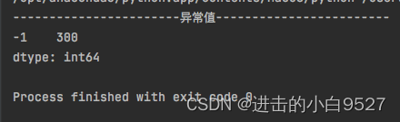
1.1 3α法则:计算数据的均值和标准差,将位于均值+/-3倍标准差之外的数据视为异常值,此种情况只是适用于正态分布 的数据
import pandas as pd
import numpy as np

data = pd.Series(np.random.randint(0, 100, size=50))
data[-1] = 300  # 设置异常值
upper_limits = np.mean(data) + 3 * np.std(data)
lower_limits = np.mean(data) - 3 * np.std(data)
cond = (data > upper_limits) | (data < lower_limits)
outlier = data[cond]
print("异常值".center(50, "-"))
print(d)
结果图:
1.2箱线图(IQR方法):绘制箱线图,根据数据的四分位数(Q1、Q3)和四分位距(IQR=Q3-Q1),将位于Q1-1.5IQR和Q3+1.5IQR之外的数据视为异常值
17.2 删除异常值
可以使用布尔索引取值和drop()方法将异常的值进行删除,删除之后索引会发生变化,需要重置索引。重置索引如果设置了inplace为True,就无返回值了。
print("异常值drop删除".center(50, "-"))
data2 = data.drop(outlier.index).reset_index(drop=True)
print(data2)
def drop(
self,
labels=None,
axis=0,
index=None,
columns=None,
level=None,
inplace=False,
errors="raise",
):
"""
Return Series with specified index labels removed.
Remove elements of a Series based on specifying the index labels.
When using a multi-index, labels on different levels can be removed
by specifying the level.
Parameters
----------
labels : single label or list-like
Index labels to drop.
axis : 0, default 0
Redundant for application on Series.
index, columns : None
Redundant for application on Series, but index can be used instead
of labels.
.. versionadded:: 0.21.0
level : int or level name, optional
For MultiIndex, level for which the labels will be removed.
inplace : bool, default False
If True, do operation inplace and return None.
errors : {'ignore', 'raise'}, default 'raise'
If 'ignore', suppress error and only existing labels are dropped.
Returns
-------
Series
Series with specified index labels removed.
Raises
------
KeyError
If none of the labels are found in the index.
See Also
--------
Series.reindex : Return only specified index labels of Series.
Series.dropna : Return series without null values.
Series.drop_duplicates : Return Series with duplicate values removed.
DataFrame.drop : Drop specified labels from rows or columns.
Examples
--------
>>> s = pd.Series(data=np.arange(3), index=['A', 'B', 'C'])
>>> s
A 0
B 1
C 2
dtype: int64
Drop labels B en C
>>> s.drop(labels=['B', 'C'])
A 0
dtype: int64
Drop 2nd level label in MultiIndex Series
>>> midx = pd.MultiIndex(levels=[['lama', 'cow', 'falcon'],
... ['speed', 'weight', 'length']],
... codes=[[0, 0, 0, 1, 1, 1, 2, 2, 2],
... [0, 1, 2, 0, 1, 2, 0, 1, 2]])
>>> s = pd.Series([45, 200, 1.2, 30, 250, 1.5, 320, 1, 0.3],
... index=midx)
>>> s
lama speed 45.0
weight 200.0
length 1.2
cow speed 30.0
weight 250.0
length 1.5
falcon speed 320.0
weight 1.0
length 0.3
dtype: float64
>>> s.drop(labels='weight', level=1)
lama speed 45.0
length 1.2
cow speed 30.0
length 1.5
falcon speed 320.0
length 0.3
dtype: float64
"""import pandas as pd
import numpy as np
data = pd.Series(np.random.randint(0, 100, size=10))
upper_limits = np.mean(data) + 3 * np.std(data)
lower_limits = np.mean(data) - 3 * np.std(data)
data.iloc[5] = 500 # 设置异常值
cond = (data > upper_limits) | (data < lower_limits)
outlier = data[cond]
print("异常值".center(50, "-"))
print(outlier)
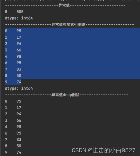
print("异常值布尔索引删除".center(50, "-"))
print(data[~cond])
print("异常值drop删除".center(50, "-"))
data.drop(outlier.index,inplace=True)
print(data)结果图:
17.3 drop函数的使用
import pandas as pd
import numpy as np
df = pd.DataFrame(
data=np.random.randint(1,10,size=(5,3)),
index=list("ABCDE"),
columns=["Python","Java","HTML"]
)
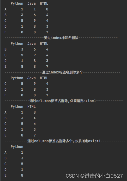
print(df)
print("通过index标签名删除".center(50,"-"))
print(df.drop("A"))
print("通过index标签名删除多个".center(50,"-"))
print(df.drop(["A","B"]))
print("通过columns标签名删除,必须指定axis=1".center(50,"-"))
print(df.drop("Java",axis=1))
print("通过columns标签名删除多个,必须指定axis=1".center(50,"-"))
print(df.drop(["Java","HTML"],axis=1))结果图:
18.map函数通过字典转换数据
18.1 字典转换数据
通过map函数将字典进行映射,将原有的数据进行替换。map()操作的对象为series.返回的对象为series.
如果series中的值,不存在映射字典中,那么series中的值就会转变为NaN
参数arg可以是 function, dict, or Series
参数na_action=ignore时,空数据,就不会被使用字典映射。
    def map(self, arg, na_action=None):
        """
        Map values of Series according to input correspondence.

        Used for substituting each value in a Series with another value,
        that may be derived from a function, a ``dict`` or
        a :class:`Series`.

        Parameters
        ----------
        arg : function, dict, or Series
            Mapping correspondence.
        na_action : {None, 'ignore'}, default None
            If 'ignore', propagate NaN values, without passing them to the
            mapping correspondence.

        Returns
        -------
        Series
            Same index as caller.

        See Also
        --------
        Series.apply : For applying more complex functions on a Series.
        DataFrame.apply : Apply a function row-/column-wise.
        DataFrame.applymap : Apply a function elementwise on a whole DataFrame.

        Notes
        -----
        When ``arg`` is a dictionary, values in Series that are not in the
        dictionary (as keys) are converted to ``NaN``. However, if the
        dictionary is a ``dict`` subclass that defines ``__missing__`` (i.e.
        provides a method for default values), then this default is used
        rather than ``NaN``.

        Examples
        --------
        >>> s = pd.Series(['cat', 'dog', np.nan, 'rabbit'])
        >>> s
        0      cat
        1      dog
        2      NaN
        3   rabbit
        dtype: object

        ``map`` accepts a ``dict`` or a ``Series``. Values that are not found
        in the ``dict`` are converted to ``NaN``, unless the dict has a default
        value (e.g. ``defaultdict``):

        >>> s.map({'cat': 'kitten', 'dog': 'puppy'})
        0   kitten
        1    puppy
        2      NaN
        3      NaN
        dtype: object

        It also accepts a function:

        >>> s.map('I am a {}'.format)
        0       I am a cat
        1       I am a dog
        2       I am a nan
        3    I am a rabbit
        dtype: object

        To avoid applying the function to missing values (and keep them as
        ``NaN``) ``na_action='ignore'`` can be used:

        >>> s.map('I am a {}'.format, na_action='ignore')
        0     I am a cat
        1     I am a dog
        2            NaN
        3  I am a rabbit
        dtype: object
        """
import pandas as pd
import numpy as np
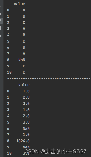
data = pd.DataFrame({"value":["A","B","C","A","B","C","D","A",np.nan,"E","C"]})
print("原始数据".center(50,"-"))
print(data)
mapping_dict = {"A":1,"B":2,"C":3,np.nan:1024}
data["value"] = data["value"].map(mapping_dict)
print("映射条件转化数据".center(50,"-"))
print(data)
data["value"] = data["value"].map('I am a {}'.format,na_action="ignore")
print("执行参数na_action".center(50,"-"))
print(data)结果图:
执行na_action:

18.2 自定义函数处理数据
import pandas as pd
import numpy as np
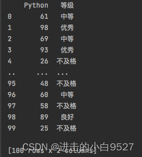
s = pd.Series(np.random.randint(0, 100, size=100), name="Python")
def covert(x):
if x < 60:
return "不及格"
elif x < 70:
return "中等"
elif x < 90:
return "良好"
else:
return "优秀"
s2 = s.map(covert)
df2 = pd.DataFrame({"Python":s,"等级":s2})
print(df2)结果图:
19.apply函数进行数据转变
19.1 applay()函数
在pandas中,apply()函数是用于Series|Dataframe的方法,它可以用于数据转换和处理。apply()接受函数作为参数,并将该函数应用到Dataframe中的每一行或每一列。
def apply(
self,
func,
axis=0,
broadcast=None,
raw=False,
reduce=None,
result_type=None,
args=(),
**kwds
):
"""
# 沿着Dataframe的轴传递函数
Apply a function along an axis of the DataFrame.
# 传递给函数的对象是series对象,其索引是Dataframe的索引(axis=1 | axis=0)
# 默认情况下(``result_type=None``),最终返回类型是从应用的函数的返回类型推断
# 出来的。否则它取决于“result_type”参数
Objects passed to the function are Series objects whose index is
either the DataFrame's index (``axis=0``) or the DataFrame's columns
(``axis=1``). By default (``result_type=None``), the final return type
is inferred from the return type of the applied function. Otherwise,
it depends on the `result_type` argument.
Parameters
----------
func : function
Function to apply to each column or row.
axis : {0 or 'index', 1 or 'columns'}, default 0
Axis along which the function is applied:
* 0 or 'index': apply function to each column.
* 1 or 'columns': apply function to each row.
broadcast : bool, optional
Only relevant for aggregation functions:
* ``False`` or ``None`` : returns a Series whose length is the
length of the index or the number of columns (based on the
`axis` parameter)
* ``True`` : results will be broadcast to the original shape
of the frame, the original index and columns will be retained.
.. deprecated:: 0.23.0
This argument will be removed in a future version, replaced
by result_type='broadcast'.
raw : bool, default False
* ``False`` : passes each row or column as a Series to the
function.
* ``True`` : the passed function will receive ndarray objects
instead.
If you are just applying a NumPy reduction function this will
achieve much better performance.
reduce : bool or None, default None
Try to apply reduction procedures. If the DataFrame is empty,
`apply` will use `reduce` to determine whether the result
should be a Series or a DataFrame. If ``reduce=None`` (the
default), `apply`'s return value will be guessed by calling
`func` on an empty Series
(note: while guessing, exceptions raised by `func` will be
ignored).
If ``reduce=True`` a Series will always be returned, and if
``reduce=False`` a DataFrame will always be returned.
.. deprecated:: 0.23.0
This argument will be removed in a future version, replaced
by ``result_type='reduce'``.
result_type : {'expand', 'reduce', 'broadcast', None}, default None
These only act when ``axis=1`` (columns):
* 'expand' : list-like results will be turned into columns.
* 'reduce' : returns a Series if possible rather than expanding
list-like results. This is the opposite of 'expand'.
* 'broadcast' : results will be broadcast to the original shape
of the DataFrame, the original index and columns will be
retained.
The default behaviour (None) depends on the return value of the
applied function: list-like results will be returned as a Series
of those. However if the apply function returns a Series these
are expanded to columns.
.. versionadded:: 0.23.0
args : tuple
Positional arguments to pass to `func` in addition to the
array/series.
**kwds
Additional keyword arguments to pass as keywords arguments to
`func`.
Returns
-------
Series or DataFrame
Result of applying ``func`` along the given axis of the
DataFrame.
See Also
--------
DataFrame.applymap: For elementwise operations.
DataFrame.aggregate: Only perform aggregating type operations.
DataFrame.transform: Only perform transforming type operations.
Notes
-----
In the current implementation apply calls `func` twice on the
first column/row to decide whether it can take a fast or slow
code path. This can lead to unexpected behavior if `func` has
side-effects, as they will take effect twice for the first
column/row.
Examples
--------
>>> df = pd.DataFrame([[4, 9]] * 3, columns=['A', 'B'])
>>> df
A B
0 4 9
1 4 9
2 4 9
Using a numpy universal function (in this case the same as
``np.sqrt(df)``):
>>> df.apply(np.sqrt)
A B
0 2.0 3.0
1 2.0 3.0
2 2.0 3.0
Using a reducing function on either axis
>>> df.apply(np.sum, axis=0)
A 12
B 27
dtype: int64
>>> df.apply(np.sum, axis=1)
0 13
1 13
2 13
dtype: int64
Returning a list-like will result in a Series
>>> df.apply(lambda x: [1, 2], axis=1)
0 [1, 2]
1 [1, 2]
2 [1, 2]
dtype: object
Passing result_type='expand' will expand list-like results
to columns of a Dataframe
>>> df.apply(lambda x: [1, 2], axis=1, result_type='expand')
0 1
0 1 2
1 1 2
2 1 2
Returning a Series inside the function is similar to passing
``result_type='expand'``. The resulting column names
will be the Series index.
>>> df.apply(lambda x: pd.Series([1, 2], index=['foo', 'bar']), axis=1)
foo bar
0 1 2
1 1 2
2 1 2
Passing ``result_type='broadcast'`` will ensure the same shape
result, whether list-like or scalar is returned by the function,
and broadcast it along the axis. The resulting column names will
be the originals.
>>> df.apply(lambda x: [1, 2], axis=1, result_type='broadcast')
A B
0 1 2
1 1 2
2 1 2
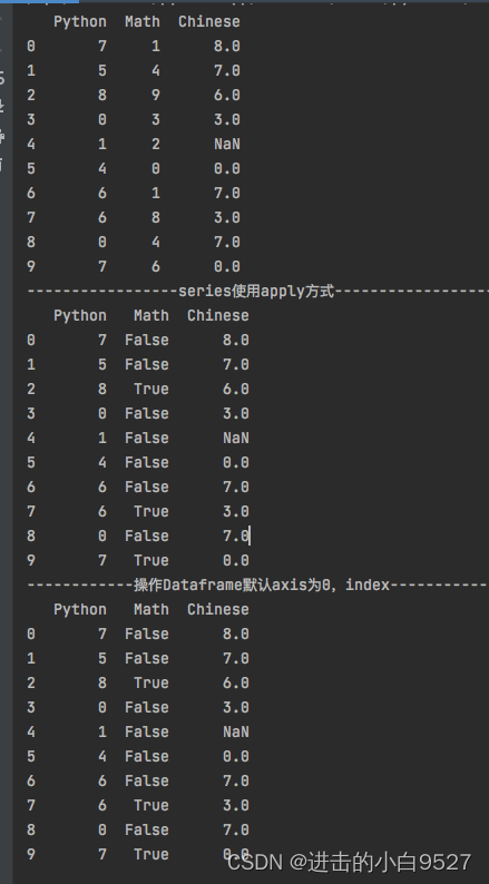
"""import pandas as pd
import numpy as np
df = pd.DataFrame(
data=np.random.randint(0, 10, size=(10, 3)),
columns=["Python", "Math", "Chinese"]
)
df.iloc[4,2] = None
print(df)
df["Math"] = df["Math"].apply(lambda x:True if x>5 else False)
print("series使用apply方式".center(50,"-"))
print(df)
df = df.apply(lambda x:x.sum(),axis=1)
print("操作Dataframe默认axis为0,index".center(50,"-"))
print(df)结果图:
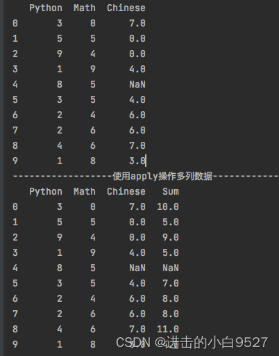
使用apply操作多列数据
import pandas as pd
import numpy as np
df = pd.DataFrame(
    data=np.random.randint(0, 10, size=(10, 3)),
    columns=["Python", "Math", "Chinese"]
)
df.iloc[4,2] = None
print(df)
def convert(row):
    return row["Python"] + row["Chinese"]
df["Sum"] = df.apply(convert,axis=1)
print("使用apply操作多列数据".center(50,"-"))
print(df)
结果图:
19.2 applymap()函数
def applymap(self, func):
"""
# 将方法应用到Dataframe上面的每一个元素
Apply a function to a Dataframe elementwise.
#此方法应用一个接受并返回标量的函数到DataFrame的每个元素。
This method applies a function that accepts and returns a scalar
to every element of a DataFrame.
Parameters
----------
func : callable
Python function, returns a single value from a single value.
Returns
-------
DataFrame
Transformed DataFrame.
See Also
--------
DataFrame.apply : Apply a function along input axis of DataFrame.
Notes
-----
In the current implementation applymap calls `func` twice on the
first column/row to decide whether it can take a fast or slow
code path. This can lead to unexpected behavior if `func` has
side-effects, as they will take effect twice for the first
column/row.
Examples
--------
>>> df = pd.DataFrame([[1, 2.12], [3.356, 4.567]])
>>> df
0 1
0 1.000 2.120
1 3.356 4.567
>>> df.applymap(lambda x: len(str(x)))
0 1
0 3 4
1 5 5
Note that a vectorized version of `func` often exists, which will
be much faster. You could square each number elementwise.
>>> df.applymap(lambda x: x**2)
0 1
0 1.000000 4.494400
1 11.262736 20.857489
But it's better to avoid applymap in that case.
>>> df ** 2
0 1
0 1.000000 4.494400
1 11.262736 20.857489
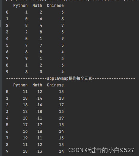
"""import pandas as pd
import numpy as np
df2 = pd.DataFrame(
data=np.random.randint(0, 10, size=(10, 3)),
columns=["Python", "Math", "Chinese"]
)
print(df2)
df2 = df2.applymap(lambda x:x+10)
print("applaymap操作每个元素".center(50,"-"))
print(df2)结果图:


 318
318


 被折叠的 条评论
为什么被折叠?
被折叠的 条评论
为什么被折叠?
 到【灌水乐园】发言


