【python】梯度下降法—线性回归

 

开始时我们随机选择一个参数的组合(θ0,θ1)，计算代价函数，然后我们寻找下一个能让代价函数值下降最多的参数组合。我们持续这么做直到到到一个局部最小值（local minimum），因为我们并没有尝试完所有的参数组合，所以不能确定我们得到的局部最小值是否便是全局最小值（global minimum），选择不同的初始参数组合，可能会找到不同的局部最小值。

其中α是学习率（learning rate），即如果步子太大了，可能会越过了最低点，如果步子太小了，则会下得慢。它决定了我们沿着能让代价函数下降程度最大的方向向下迈出的步子有多大，在批量梯度下降中，我们每一次都同时让所有的参数减去学习速率乘以代价函数的导数，以此来更新参数，参数必须要同时更新。

import numpy as np
import matplotlib.pyplot as plt
from sympy import symbols, diff

def costFunctionJ(x, y, theta):
    '''代价函数'''——最小化，形式为均方误差乘以1/2，用来抵消平方求导，方便求导，但我们使用的是一般求导方法
    a =0
    b =0
    for i in range(len(x)):
        prediction = x[i] * theta[1] + theta[0]
        a += (prediction - y[i]) ** 2
        b += 1
    Errors=1/2*(a/b)
    return Errors


def gradientDescent(x, y, theta, alpha, num_iters):
    '''
    alpha为学习率
    num_iters为迭代次数
    '''
    m = len(y)
    n = len(theta)
    temp = np.mat(np.zeros([n, num_iters]))  # 用来暂存每次迭代更新的theta值，是一个矩阵形式
    j_history = np.mat(np.zeros([num_iters, 1]))  # #记录每次迭代计算的代价值
    for i in range(num_iters):  # 遍历迭代次数
        # 定义变量和函数
        theta_0 = symbols('theta_0')
        theta_1 = symbols('theta_1')
        # 求偏导
        derivative_0 = diff(costFunctionJ(x, y, [theta_0,theta_1]), theta_0).subs({theta_0: theta[0], theta_1: theta[1]})
        derivative_1 = diff(costFunctionJ(x, y, [theta_0, theta_1]), theta_1).subs(
            {theta_0: theta[0], theta_1: theta[1]})
        theta = np.array(theta) - alpha* np.array([derivative_0,derivative_1]) # 更新参数
        temp[:, i] = np.mat(theta).T
        theta=theta.tolist()
        j_history[i] = costFunctionJ(x, y, theta)
    return theta, j_history, temp


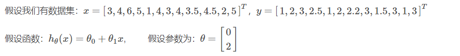
x = [3,4,6,5,1,4,3,4,3.5,4.5,2,5]
theta = [0, 2]  # 给定初始参数
y = [1, 2, 3, 2.5, 1, 2, 2.2, 3, 1.5, 3, 1, 3]

# 求代价函数值
j = costFunctionJ(x, y, theta)
# print('代价值：',j)

plt.figure(figsize=(15, 5))
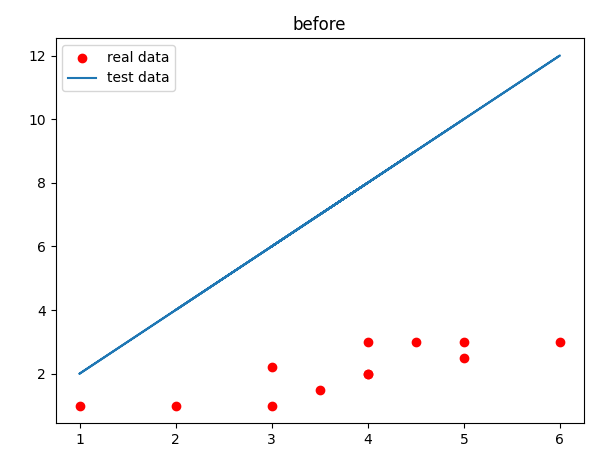
plt.subplot(1, 2, 1)
plt.scatter(x, y, c='r', label='real data')  # 画梯度下降前的图像
plt.plot(x, np.array(x) * theta[1]+theta[0], label='test data')
plt.legend(loc='best')
plt.title('before')

theta, j_history, temp = gradientDescent(x, y, theta, 0.01, 100)
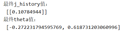
print('最终j_history值：\n', j_history[-1])
print('最终theta值：\n', theta)
print('每次迭代的代价值：\n', j_history)
print('theta值更新历史：\n', temp)

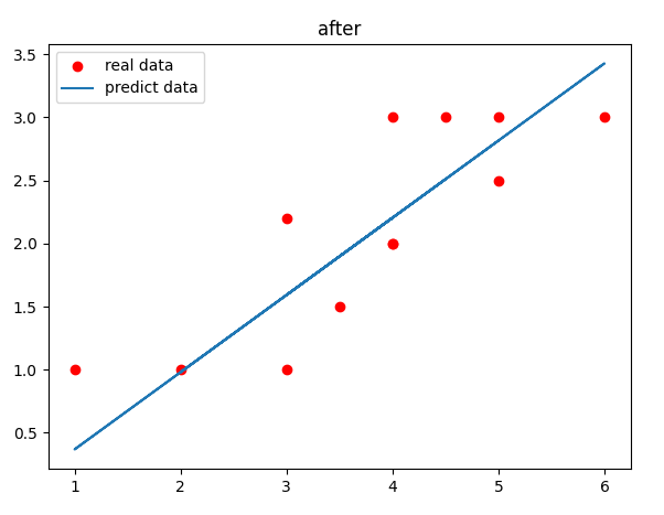
plt.subplot(1, 2, 2)
plt.scatter(x, y, c='r', label='real data')  # 画梯度下降后的图像
plt.plot(x, np.array(x) * theta[1]+theta[0], label='predict data')
plt.legend(loc='best')
plt.title('after')
plt.show()

 

 

---

参考： python实现线性回归梯度下降法（吴恩达机器学习—笔记）_线性回归梯度下降python-CSDN博客