tensor基础语法（深度学习）

皓鹏飞

已于 2024-05-23 18:01:19 修改

阅读量608

点赞数 25

文章标签：深度学习人工智能

于 2024-05-15 23:03:25 首次发布

本文链接：https://blog.csdn.net/m0_72678524/article/details/138808434

版权

tensor

torch.tensor是包含单一数据类型元素的多维数组，他是PyTorch中数据存储和运算的基本单元，类似于numpy的numpy.ndarray,两者的函数接口和运算方式几乎一样。实际上PyTorch内部也是把ndarray包装成Tensor。

Tensor中文称为张量（就相当于高维度的数组，3维及3维以上应该是属于高维数组了），是PyTorch中最基本的数据类型。在数学中，标量只有大小没有方向，向量有大小有方向，矩阵是多个向量组成的二维数组。实际上，标量，向量和矩阵都可以看作是张量的特例，标量是0维的，向量是1维的，矩阵是2维的。

1.tensor的使用

1.1tensor的创建

通过列表创建

x = torch.tensor([1,2])
print(x)

通过元组创建

x = torch.tensor((1, 2))
print(x)

通过numpy创建

import numpy as np
n = np.array([1, 2])
x = torch.tensor(n)
print(x)

1.2张量的维度

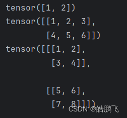
如下所示：

# 一维向量
t1 = torch.tensor((1, 2))
# 二维向量
t2 = torch.tensor([[1, 2, 3], [4, 5, 6]])
# 三维向量
t3 = torch.tensor([[[1, 2], [3, 4]],[[5, 6], [7, 8]]])

运行结果

1.3查看张量维度

ndim返回的是数组的维度，返回的只有一个数，该数即表示数组的维度。

print(t1.ndim, t2.ndim, t3.ndim, sep = ', ')
# 1, 2, 3
# t1为1维向量
# t2为2维矩阵
# t3为3维张量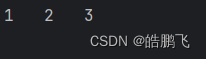

1.4查看向量的形状

size() 函数返回一个包含张量每个维度大小的列表。对于一维张量（向量），它将返回一个元素的列表，表示向量的长度。对于二维张量（矩阵），它将返回一个包含两个元素的列表，分别表示矩阵的行数和列数。对于更高维度的张量，列表的长度将相应增加。

以二维矩阵举例：

import torch  
A = torch.tensor([[1, 2, 3], [4, 5, 6]])  
x = A.size()  
print(x)  
#输出: torch.Size([2, 3])

shape 函数返回一个表示数组或张量各个维度大小的元组。对于一维数组（或称为向量），shape 将返回一个只包含一个元素的元组，表示数组的长度。对于二维数组（或称为矩阵），shape 将返回一个包含两个元素的元组，分别表示矩阵的行数和列数。对于更高维度的数组或张量，shape 返回的元组将包含相应数量的元素。

import numpy as np  
# 一维数组  
a = np.array([1, 2, 3, 4, 5])  
print(a.shape)  
# 输出: (5,)  
# 二维数组（矩阵）  
b = np.array([[1, 2, 3], [4, 5, 6]])  
print(b.shape)  
# 输出: (2, 3)  
# 三维数组  
c = np.array([[[1, 2], [3, 4]], [[5, 6], [7, 8]]])  
print(c.shape)  
# 输出: (2, 2, 2)

1.5查看张量中的元素个数

在深度学习和数值计算中，numel 函数（在 MATLAB 和一些类似的工具中）用于计算数组或张量中元素的总数。在 Python 的 NumPy 库中，虽然没有一个直接名为 numel 的函数，但你可以使用 size 函数（不带参数）或 numpy.prod 函数（计算数组中所有维度大小的乘积）来达到类似的效果。

在 PyTorch 中，也没有直接名为 numel 的函数，但 PyTorch 的张量（Tensor）有一个 .numel() 方法，它返回张量中元素的数量。

import torch  
# 创建一个二维张量（类似于矩阵）  
tensor = torch.tensor([[1, 2, 3], [4, 5, 6]])  
# 使用 .numel() 方法来计算元素总数  
num_elements = tensor.numel()  
print(num_elements)  
# 输出: 6

1.6索引和切片

import torch  
# 创建一个一维Tensor  
x = torch.tensor([1, 2, 3, 4, 5])  
# 索引  
print(x[0])  
# 输出: tensor(1)  
# 切片  
print(x[1:4])  
# 输出: tensor([2, 3, 4])

二维tensor

# 创建一个二维Tensor  
x = torch.tensor([[1, 2, 3], [4, 5, 6], [7, 8, 9]])   
# 索引（行和列）  
print(x[0, 1])  
# 输出: tensor(2)  
# 切片（行）  
print(x[0:2, :])  
# 输出:   
# tensor([[1, 2, 3],  
#         [4, 5, 6]])  
# 切片（列）  
print(x[:, 1:3])  
# 输出:   
# tensor([[2, 3],  
#         [5, 6],  
#         [8, 9]])  
# 索引和切片组合  
print(x[1:, 1:3])  
# 输出:   
# tensor([[5, 6],  
#         [8, 9]])

更高维度的操作，索引和操作类似

注意：在切片时，如果省略了开始索引，它默认为0；如果省略了结束索引，它默认为Tensor的最后一个索引。

1.7tensor的连接

使用torch.cat()函数，可以在指定的维度上将多个Tensor连接起来。这个函数需要两个主要参数：要连接的Tensor列表（tensors）和连接的维度（dim）。

import torch  
a = torch.rand(4, 32, 8)  
b = torch.rand(5, 32, 8)  
c = torch.cat([a, b], dim=0) 
#dim就是代表的那个维度 
# 在0维度上连接a和b，
# c的形状为[9, 32, 8]
# 运行结果： torch.Size([9, 32, 8])

1.8tensor的拆分

PyTorch提供了多种函数用于拆分Tensor，例如torch.chunk()、torch.split()等。torch.chunk()函数将一个Tensor拆分成指定数量的块，并返回一个新的Tensor列表。

d = torch.rand(9, 32, 8)  
e = torch.chunk(d, 3, dim=0)  
# 将d在0维度上拆分成3块，e是一个包含3个Tensor的列表

torch.split()和torch.chunk() 类似，但torch.split()比torch.chunk()使用更加细致一些，能够控制每一个块的大小。

1.9tensor的换位和置换

在PyTorch中，Tensor的换位和置换通常指的是改变Tensor的维度顺序。

transpose(dim0, dim1)：这个函数将输入Tensor的dim0和dim1两个维度进行交换。其他维度的顺序保持不变。（这个函数只能处理二维问题）

permute()：该函数可以随意交换任意维度，并且可以重新排列整合维度。（这个函数可以处理高维问题）

1.10tensor的运算

加减乘除

示例：（乘法是以点乘举例）

t1 = torch.full(size=(3,4),fill_value=2)
t2 = 2

# 加
out1 = t1 + t2
out2 = torch.add(t1, t2)

# 减
out3 = t1 - t2
out4 = torch.sub(t1, t2)

# 乘
out5 = t1 * t2
out6 = torch.mul(t1, t2)

# 除
out7 = t1 / t2
out8 = torch.div(t1, t2)

print(t1)
print(t1.shape)
print()

print(out1)
print(out1.shape)
print()
print(out2)
print(out2.shape)
print()

print(out3)
print(out3.shape)
print()
print(out4)
print(out4.shape)
print()

print(out5)
print(out5.shape)
print()
print(out6)
print(out6.shape)
print()

print(out7)
print(out7.shape)
print()
print(out8)
print(out8.shape)
# 进行tensor的加减乘除运算时有一个broadcasting（广播）进行
# 输出结果:
# tensor([[2, 2, 2, 2],
#         [2, 2, 2, 2],
#         [2, 2, 2, 2]])
# torch.Size([3, 4])

# 加
# tensor([[4, 4, 4, 4],
#         [4, 4, 4, 4],
#         [4, 4, 4, 4]])
# torch.Size([3, 4])
# 
# tensor([[4, 4, 4, 4],
#         [4, 4, 4, 4],
#         [4, 4, 4, 4]])
# torch.Size([3, 4])

# 减 
# tensor([[0, 0, 0, 0],
#         [0, 0, 0, 0],
#         [0, 0, 0, 0]])
# torch.Size([3, 4])
# 
# tensor([[0, 0, 0, 0],
#         [0, 0, 0, 0],
#         [0, 0, 0, 0]])
# torch.Size([3, 4])

# 乘 
# tensor([[4, 4, 4, 4],
#         [4, 4, 4, 4],
#         [4, 4, 4, 4]])
# torch.Size([3, 4])
# 
# tensor([[4, 4, 4, 4],
#         [4, 4, 4, 4],
#         [4, 4, 4, 4]])
# torch.Size([3, 4])

# 除 
# tensor([[1., 1., 1., 1.],
#         [1., 1., 1., 1.],
#         [1., 1., 1., 1.]])
# torch.Size([3, 4])
# 
# tensor([[1., 1., 1., 1.],
#         [1., 1., 1., 1.],
#         [1., 1., 1., 1.]])
# torch.Size([3, 4])

矩阵乘法

torch.mm:矩阵相乘，要求a的列数和b的行数相同且不支持广播机制。

import torch
t1 = torch.rand(3,4)
t2 = torch.rand(4,2)
print(t1)
print()
print(t2)
print()
out1 = torch.mm(t1, t2)
out2 = t1 @ t2
print(out1)
print()
print(out2)
# t1
# tensor([[0.9025, 0.1912, 0.0642, 0.0823],
#         [0.3470, 0.4985, 0.3564, 0.5059],
#         [0.1635, 0.6606, 0.4504, 0.4293]])
# t2
# tensor([[0.6877, 0.2833],
#         [0.2483, 0.3837],
#         [0.2300, 0.8279],
#         [0.2310, 0.5820]])
# out1
# tensor([[0.7019, 0.4301],
#         [0.5612, 0.8791],
#         [0.4792, 0.9226]])
# out2
# tensor([[0.7019, 0.4301],
#         [0.5612, 0.8791],
#         [0.4792, 0.9226]])

torch.mul:矩阵的对应位置相乘，a和b的维度必须保持一致。

import torch
t1 = torch.rand(3,4)
t2 = torch.rand(3,4)
print(t1)
print()
print(t2)
print()
out1 = torch.mul(t1, t2)
out2 = t1 * t2
print(out1)
print()
print(out2)
# tensor([[0.6266, 0.3121, 0.5366, 0.3205],
#         [0.1849, 0.4022, 0.7654, 0.0840],
#         [0.9421, 0.2146, 0.3300, 0.4202]])
# 
# tensor([[0.3330, 0.6612, 0.5825, 0.0350],
#         [0.3143, 0.4830, 0.6548, 0.4956],
#         [0.6734, 0.3350, 0.0947, 0.4882]])
# 
# tensor([[0.2087, 0.2064, 0.3126, 0.0112],
#         [0.0581, 0.1942, 0.5012, 0.0416],
#         [0.6345, 0.0719, 0.0312, 0.2051]])
# 
# tensor([[0.2087, 0.2064, 0.3126, 0.0112],
#         [0.0581, 0.1942, 0.5012, 0.0416],
#         [0.6345, 0.0719, 0.0312, 0.2051]])

torch.matmul:没有强制规定维度和大小，可以使用广播机制进行不同维度的相乘操作。

import torch
t1 = torch.rand(2,3)
t2 = torch.rand(3,4)
print(t1)
print()
print(t2)
print()
out1 = torch.matmul(t1, t2)
print(out1)
# tensor([[0.3842, 0.8509, 0.6124],
#        [0.1927, 0.9945, 0.4779]])
#
# tensor([[0.4128, 0.8906, 0.2295, 0.5790],
#        [0.9892, 0.7096, 0.6086, 0.0796],
#        [0.6981, 0.2769, 0.6924, 0.6392]])
#
# tensor([[1.4279, 1.1156, 1.0301, 0.6817],
#        [1.3969, 1.0096, 0.9804, 0.4962]])

皓鹏飞

关注

25
点赞
踩
10

收藏

觉得还不错? 一键收藏
0
评论
tensor基础语法（深度学习）

实际上，标量，向量和矩阵都可以看作是张量的特例，标量是0维的，向量是1维的，矩阵是2维的。torch.tensor是包含单一数据类型元素的多维数组，他是PyTorch中数据存储和运算的基本单元，类似于numpy的numpy.ndarray,两者的函数接口和运算方式几乎一样。对于一维张量（向量），它将返回一个元素的元组，表示向量的长度。对于二维张量（矩阵），它将返回一个包含两个元素的元组，分别表示矩阵的行数和列数。对于更高维度的数组或张量，ndim返回的是数组的维度，返回的只有一个数，该数即表示数组的维度。
复制链接

扫一扫