逻辑回归及其python实现

1. 二分类逻辑回归

$$\begin{gathered} z=\vec{x}\vec{w}=w_0+w_1{x}_1+w_2{x}_2+...+w_n{x}_n \\ y=h_w(x)=sigmoid(z)=\frac{1}{1+e^{-z}} \end{gathered}$$

(1). 交叉熵损失函数

$$J(w)=-\frac{1}{m}\sum _{i=1}^m[y^{(i)}log({\hat{y}}^{(i)})+(1-y^{(i)})log(1-{\hat{y}}^{(i)})]$$

(2). 交叉熵损失函数原理推导

交叉熵损失函数的本质是等价于极大似然估计，已知：
$$\begin{gathered} P(y=1|x,w)=h_w(x) \\ P(y-0|x,w)=1-h_w(x) \end{gathered}$$
因此
$$P(y|x,w)=h_w(x{)}^y(1-h_w(x){)}^{1-y}$$
极大似然函数
$$L(w)=\prod _{i=1}^m{h}_w(x^{(i)}{)}^{y^{(i)}}(1-h_w(x^{(i)}){)}^{1-y^{(i)}}$$
对极大似然函数取对数然后取反，即得交叉熵损失函数（为了样本规模影响loss大小，损失函数除以了m），因此最小化交叉熵损失函数等价于最大化极大似然函数

(3). 梯度下降

(i). 偏导

$$\frac{\partial J}{\partial w}=\frac{1}{m}\sum _{i=1}^m({\hat{y}}^{(i)}-y^{(i)})x^{(i)}=\frac{1}{m}{X}^T(h_w(X)-\vec{y})$$

(ii). 参数更新

$$w=w-\alpha \ast \frac{\partial J}{\partial w}$$

2. 多元逻辑回归

• one vs rest 考虑某种类型为正值1，其余全为0，训练K个logistic分类器，适合K个类型不互斥的情况
• one vs one: 选择一个类别和另一个类别训练分类器， softmax 多元逻辑回归

(1). softmax 多元逻辑回归

$$P(y=k|x,w)=\frac{e^{x{w}_k}}{{\sum }_{t=1}^K{e}^{x{w}_t}}$$

其中$w_{K\ast n}$

(2). 损失函数

$$J(w)=-\sum _{i=1}^m\sum _{t=1}^K{1}_{y=j}log(P(y=t|x,w))$$

3. python 实现

import numpy as np
import matplotlib.pyplot as plt
from sklearn import datasets

def sigmoid(z):
    return (1/(1+np.exp(-z)))


def model(X, theta):
    """
    X array(m * n)
    theta array(n * 1)
    
    return : array (m * 1)
    """
    return sigmoid(X @ theta)


def computerCost(X, y, theta):
    """
    X: array(m * n)
    y: array(m * 1)
    theta: array(n * 1)
    """
    y_pred = model(X, theta)
    m = X.shape[0]
    J = (-1/m) * (y.T @ np.log(y_pred) +(1-y.T) @ np.log(1-y_pred))
    return np.squeeze(J)


def gradientDescent(X, y, theta, alpha, num_iters):
    '''
    X: array(m * n)
    y: array(m * 1)
    theta: array(n * 1)
    alpha: learning rate between (0, 1)
    num_iters: number of iteration times
    
    n should be the feature number plus 1
    '''
    J_history = np.empty((num_iters, 1))
    for i in range(num_iters):
        theta = theta - alpha * (1/m * (X.T @ (model(X, theta) - y)))
        J_history[i] = computerCost(X, y, theta)
        print('.', end='')
    return theta, J_history
    
# 多元分类
def one_vs_all(X, y, k, theta, alpha, num_iters):
    
    J_history = np.empty((k, num_iters, 1))
 
    # 训练k个分类器
    for i in range(k):
        y_k = (y==i)
        theta_k = theta[:, i]
        theta_k = theta_k[:, np.newaxis]
        theta_k, J_history[i, :, :] = gradientDescent(X, y_k, theta_k, alpha, num_iters)
        theta[:, i] = np.squeeze(theta_k)
        print('\n**************\n')

        
    return theta, J_history


def predict(X, theta):
    y_pred = model(X, theta)
    y_type = np.argmax(y_pred, axis=1)
    return y_type[:, np.newaxis]

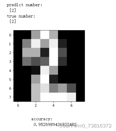
1. 一个实例：手写数字识别

digits = datasets.load_digits()
X = digits.data
y = digits.target
m = len(y)
n = X.shape[1] + 1
X_adjust = np.hstack((np.ones((m, 1)), X))
y = np.expand_dims(y, axis=1)

k = 10
alpha = 0.1
num_iters = 100
theta = np.random.random((n, k))

theta, J_history = one_vs_all(X_adjust, y, k, theta, alpha, num_iters)

# 随意选择一个数据观察预测值和真实值，并可视化该手写数字灰度图
pick_index = 268
x = X[pick_index, :]
x_adjust = np.expand_dims(x, axis=0)
x_adjust = np.hstack((np.ones((1, 1)), x_adjust))
y_pred = predict(x_adjust, theta)
plt.imshow(digits.images[pick_index], cmap='gray')
print("predict number:\n", y_pred)
print("true number:\n", y[pick_index])

# 计算准确率
y_pred = predict(X_adjust, theta)
accuracy = np.sum((y_pred == y)) / len(y)
print(accuracy)

2. 结果