电子运动及电子比荷测量

中南民族大学-大学物理实验2-2024-通信工程

---

代码实现

import seaborn as sns
import matplotlib.pyplot as plt
from scipy.stats import linregress

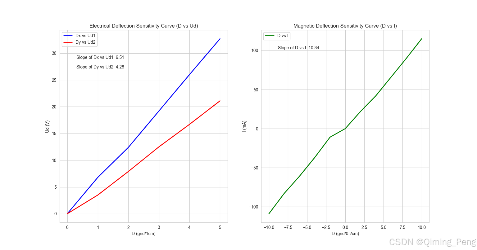
# 电偏转灵敏度
Dx = [0, 1, 2, 3, 4, 5]
Ud1 = [0, 6.8, 12.4, 19.2, 26.0, 32.7]

Dy = [0, 1, 2, 3, 4, 5]
Ud2 = [0, 3.5, 7.9, 12.5, 16.7, 21.1]

# 磁偏转灵敏度
D = [-10, -8, -6, -4, -2, 0, 2, 4, 6, 8, 10]
I = [-109, -83, -61, -37, -11, 0, 22, 42, 66, 90, 115]

# 使用 Seaborn 绘制曲线
sns.set_style("whitegrid")
fig, (ax1, ax2) = plt.subplots(1, 2, figsize=(16, 6))

# 绘制 Dx 和 Ud1 的曲线
sns.lineplot(x=Dx, y=Ud1, color='b', linewidth=2, label='Dx vs Ud1', ax=ax1)
ax1.set_title("Electrical Deflection Sensitivity Curve (D vs Ud)")
ax1.set_xlabel("D (grid/1cm)")
ax1.set_ylabel("Ud (V)")

# 绘制 Dy 和 Ud2 的曲线
sns.lineplot(x=Dy, y=Ud2, color='r', linewidth=2, label='Dy vs Ud2', ax=ax1)
ax1.legend()

# 计算斜率并显示
slope1, intercept1, r_value1, p_value1, std_err1 = linregress(Dx, Ud1)
slope2, intercept2, r_value2, p_value2, std_err2 = linregress(Dy, Ud2)
ax1.text(0.1, 0.85, f"Slope of Dx vs Ud1: {slope1:.2f}", transform=ax1.transAxes)
ax1.text(0.1, 0.80, f"Slope of Dy vs Ud2: {slope2:.2f}", transform=ax1.transAxes)

# 绘制 D 和 I 的曲线
sns.lineplot(x=D, y=I, color='g', linewidth=2, label='D vs I', ax=ax2)
ax2.set_title("Magnetic Deflection Sensitivity Curve (D vs I)")
ax2.set_xlabel("D (grid/0.2cm)")
ax2.set_ylabel("I (mA)")

# 计算斜率并显示
slope3, intercept3, r_value3, p_value3, std_err3 = linregress(D, I)
ax2.text(0.1, 0.9, f"Slope of D vs I: {slope3:.2f}", transform=ax2.transAxes)

# 显示图形
plt.show()

结果显示

 

总结 

豆包MarsCode给予了非常大的帮助，所有代码几乎都是生成的。我只知道 seaborn 这个库，其余都交给它了。还会给我补充标题、注释等细节，非常强大！👍