用python+numpy+matplotalib实现梯度下降法

这个阶段一直在做和梯度一类算法相关的东西，索性在这儿做个汇总，

一、算法论述

梯度下降法(gradient  descent)别名最速下降法（曾经我以为这是两个不同的算法-.-）,是用来求解无约束最优化问题的一种常用算法。下面以求解线性回归为题来叙述：

设：一般的线性回归方程（拟合函数）为：（其中的值为1）

  

则这一组向量参数选择的好与坏就需要一个机制来评估，据此我们提出了其损失函数为(选择均方误差)：

我们现在的目的就是使得损失函数取得最小值，即目标函数为：

如果的值取到了0，意味着我们构造出了极好的拟合函数，也即选择出了最好的值，但这基本是达不到的，我们只能使得其无限的接近于0，当满足一定精度时停止迭代。

那么问题来了如何调整使得取得的值越来越小呢？方法很多，此处以梯度下降法为例：

分为两步：（1）初始化的值。

                  （2）改变的值，使得按梯度下降的方向减少。

值的更新使用如下的方式来完成：

        

其中为步长因子，这里我们取定值，但注意如果取得过小会导致收敛速度过慢，过大则损失函数可能不会收敛，甚至逐渐变大，可以在下述的代码中修改的值来进行验证。后面我会再写一篇关于随机梯度下降法的文章，其实与梯度下降法最大的不同就在于一个求和符号。

 

二、代码实现：

import numpy as np
import matplotlib.pyplot as plt
from mpl_toolkits.mplot3d import axes3d
from matplotlib import style


#构造数据
def get_data(sample_num=10000):
    """
    拟合函数为
    y = 5*x1 + 7*x2
    :return:
    """
    x1 = np.linspace(0, 9, sample_num)
    x2 = np.linspace(4, 13, sample_num)
    x = np.concatenate(([x1], [x2]), axis=0).T
    y = np.dot(x, np.array([5, 7]).T)  
    return x, y
#梯度下降法
def GD(samples, y, step_size=0.01, max_iter_count=1000):
    """
    :param samples: 样本
    :param y: 结果value
    :param step_size: 每一接迭代的步长
    :param max_iter_count: 最大的迭代次数
    :param batch_size: 随机选取的相对于总样本的大小
    :return:
    """
    #确定样本数量以及变量的个数初始化theta值
    m, var = samples.shape
    theta = np.zeros(2)
    y = y.flatten()
    #进入循环内
    print(samples)
    loss = 1
    iter_count = 0
    iter_list=[]
    loss_list=[]
    theta1=[]
    theta2=[]
    #当损失精度大于0.01且迭代此时小于最大迭代次数时，进行
    while loss > 0.001 and iter_count < max_iter_count:
        loss = 0
        #梯度计算
        theta1.append(theta[0])
        theta2.append(theta[1])
        for i in range(m):
            h = np.dot(theta,samples[i].T)   
        #更新theta的值,需要的参量有：步长，梯度
            for j in range(len(theta)):
                theta[j] = theta[j] - step_size*(1/m)*(h - y[i])*samples[i,j]
        #计算总体的损失精度，等于各个样本损失精度之和
        for i in range(m):
            h = np.dot(theta.T, samples[i])
            #每组样本点损失的精度
            every_loss = (1/(var*m))*np.power((h - y[i]), 2)
            loss = loss + every_loss

        print("iter_count: ", iter_count, "the loss:", loss)
        
        iter_list.append(iter_count)
        loss_list.append(loss)
        
        iter_count += 1
    plt.plot(iter_list,loss_list)
    plt.xlabel("iter")
    plt.ylabel("loss")
    plt.show()
    return theta1,theta2,theta,loss_list
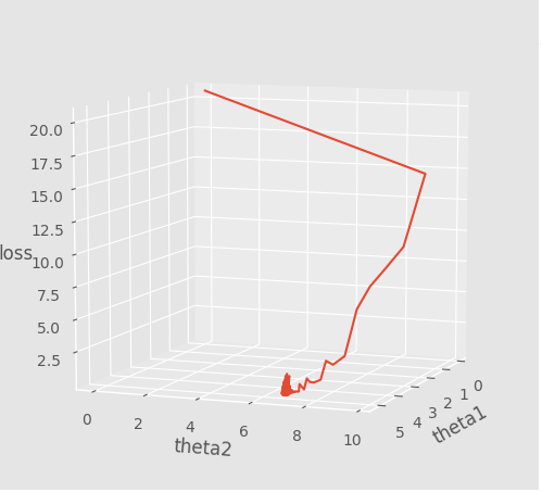
def painter3D(theta1,theta2,loss):
    style.use('ggplot')
    fig = plt.figure()
    ax1 = fig.add_subplot(111, projection='3d')
    x,y,z = theta1,theta2,loss
    ax1.plot_wireframe(x,y,z, rstride=5, cstride=5)
    ax1.set_xlabel("theta1")
    ax1.set_ylabel("theta2")
    ax1.set_zlabel("loss")
    plt.show()
def predict(x, theta):
    y = np.dot(theta, x.T)
    return y        
if __name__ == '__main__':
    samples, y = get_data()
    theta1,theta2,theta,loss_list = GD(samples, y)
    print(theta)  # 会很接近[5, 7] 
    painter3D(theta1,theta2,loss_list)
    predict_y = predict(theta, [7,8])
    print(predict_y)

三、绘制的图像如下：

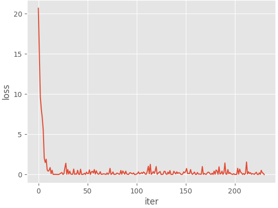
迭代次数与损失精度间的关系图如下：步长为0.01

变量、与损失函数loss之间的关系：（从初始化之后会一步步收敛到loss满足精度，之后、会变的稳定下来）

下面我们来看一副当步长因子变大后的图像：步长因子为0.5（很明显其收敛速度变缓了）

当步长因子设置为1.8左右时，其损失值已经开始震荡