ML机器学习基于树的家族

最新推荐文章于 2024-06-18 16:19:01 发布

ma416539432

最新推荐文章于 2024-06-18 16:19:01 发布

阅读量916

点赞数

分类专栏：机器学习实践机器学习原理文章标签：机器学习算法

本文链接：https://blog.csdn.net/ma416539432/article/details/53216055

版权

机器学习实践同时被 2 个专栏收录

4 篇文章 0 订阅

订阅专栏

机器学习原理

4 篇文章 0 订阅

订阅专栏

ML机器学习基于树的家族

决策树模型与学习
特征选择
决策树的生成
3.1 决策树的编程实现
3.2 画出决策树的方式
决策树的剪枝
DBGT
随机森林

参考资料：
机器学习实战
统计学习方法李航
博客
http://www.cnblogs.com/maybe2030/

–

1）决策树模型与学习

我们来谈一谈机器学习算法中的各种树形算法，包括ID3、C4.5、CART以及基于集成思想的树模型Random Forest和GBDT。本文对各类树形算法的基本思想进行了简单的介绍，重点谈一谈被称为是算法中的“战斗机”，机器学习中的“屠龙刀”的GBDT算法。
决策树根据一步步地属性分类可以将整个特征空间进行划分，从而区别出不同的分类样本，如下图所示：
这里写图片描述
根据上图其实我们不难可以想到，满足样本划分的决策树有无数种，什么样的决策树才算是一颗好的决策树呢？

性能良好的决策树的选择标准是一个与训练数据矛盾较小的决策树，同时具有很好的泛化能力。言外之意就是说，好的决策树不仅对训练样本有着很好的分类效果，对于测试集也有着较低的误差率。
决策树的优点
1、推理过程容易理解,决策推理过程可以表示成If Then
形式;
2、推理过程完全依赖于属性变量的取值特点;
3、可自动忽略目标变量没有贡献的属性变量,也为判断
属性变量的重要性,减少变量的数目提供参考，可以用来处理特征工程

与决策树相关的重要算法包括:
CLS, ID3,C4.5,CART
算法的发展过程
Hunt,Marin和Stone 于1966年研制的CLS学习系统,用于学习单个概
念。
1979年, J.R. Quinlan 给出ID3算法,并在1983年和1986年对ID3 进行了
总结和简化,使其成为决策树学习算法的典型。
Schlimmer 和Fisher 于1986年对ID3进行改造,在每个可能的决策树节
点创建缓冲区,使决策树可以递增式生成,得到ID4算法。
1988年,Utgoff 在ID4基础上提出了ID5学习算法,进一步提高了效率。
1993年,Quinlan 进一步发展了ID3算法,改进成C4.5算法。

另一类决策树算法为CART,与C4.5不同的是,CART的决策树由二元
逻辑问题生成,每个树节点只有两个分枝,分别包括学习实例的正例

一个完整的决策树学习算法包含有三大步骤，分别为：

1) 特征的选择；
　　2) 决策树的生成；
　　3) 决策树的剪枝。

2）特征选择

1) 熵（entropy）

在信息论和概率统计中，熵是表示随机变量不确定性的度量。
　　这里写图片描述

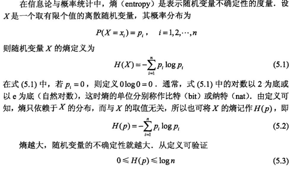
熵只依赖X的分布，和X的取值没有关系，熵是用来度量不确定性，当熵越大，概率说X=xi的不确定性越大，反之越小，在机器学期中分类中说，熵越大即这个类别的不确定性更大，反之越小，当随机变量的取值为两个时，熵随概率的变化曲线如下图：
　　这里写图片描述
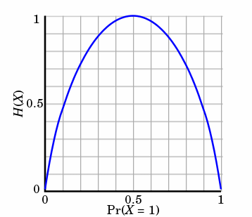
　　当p=0或p=1时，H§=0,随机变量完全没有不确定性，当p=0.5时，H§=1,此时随机变量的不确定性最大。

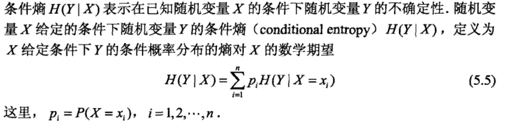
条件熵（conditional entropy）：表示在给定随机变量X的条件下随机变量Y的不确定性度量。

这里写图片描述

2) 信息增益（information gain）

这里写图片描述

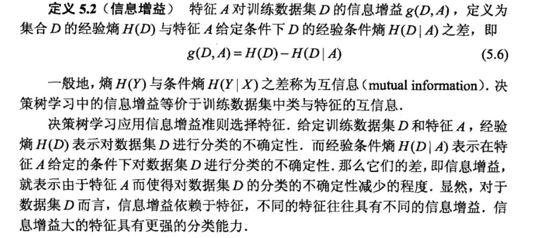
3) 信息增益比（information gain ratio）
　这里要重点关注一下这个地方，C4.5和ID3算法的不同之处就在此，ID3算法用信息增益来选择划分数据空间的特征，而C4.5用信息增益比来选择来划分空间的特征，是对ID3算法的改进。
这里写图片描述

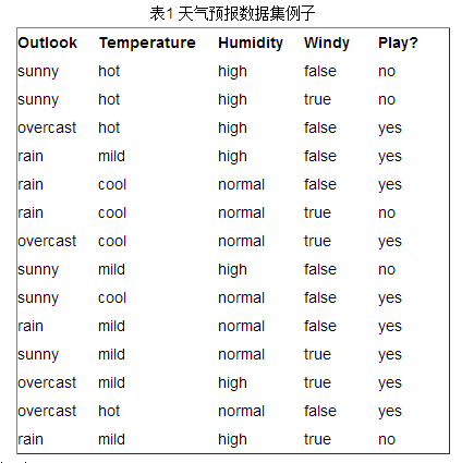
在这个例子中，最后一列指是否出去玩，这里作为我们所要预测的标记值（label），而前四列就是我们需要借助的数据，每一列都是一个特征（feature）。
初始状态下，label列总共为14行，有9个yes和5个no，所以label列初始信息熵为：
[外链图片转存失败,源站可能有防盗链机制,建议将图片保存下来直接上传(img-Aq9wQS8N-1635756835437)(https://zhihu.com/equation?tex=E%28S%29=-%5Cfrac%7B9%7D%7B14%7Dlog_%7B2%7D%28%5Cfrac%7B9%7D%7B14%7D%29-%20%5Cfrac%7B5%7D%7B14%7Dlog_%7B2%7D%28%5Cfrac%7B5%7D%7B14%7D%29)]

假设我们先划分outlook这一列，分成sunny、rain、overcast三类，数量分别为5：5：4，考虑到每个类别下对应的label不同，可以计算出划分后的信息熵：
[外链图片转存失败,源站可能有防盗链机制,建议将图片保存下来直接上传(img-bdzMHH79-1635756835439)(https://zhihu.com/equation?tex=E%28A%29=%5Csum_%7Bv%5Cin%20value%28A%29%7D%7B%5Cfrac%7Bnum%28S_%7Bv%7D%29%20%7D%7Bnum%28S%29%7DE%28S_%7Bv%7D%20%29%20%7D%20)]
[外链图片转存失败,源站可能有防盗链机制,建议将图片保存下来直接上传(img-1gJjILqQ-1635756835439)(https://zhihu.com/equation?tex=E%28A%29=%5Cfrac%7B5%7D%7B14%7DE%28S_%7B1%7D%20%29%2b%5Cfrac%7B5%7D%7B14%7DE%28S_%7B2%7D%20%29%2b%5Cfrac%7B4%7D%7B14%7DE%28S_%7B3%7D%20%29%20%20%20)]
其中E(S1)、E(S2)、E(S3)分别为每个类别下对应的label列的熵。

而信息增益（Info-Gain）就是指划分前后信息熵的变化：
[外链图片转存失败,源站可能有防盗链机制,建议将图片保存下来直接上传(img-aMz56G8f-1635756835442)(https://zhihu.com/equation?tex=IGain%28S,A%29=E%28S%29-E%28A%29)]
在ID3算法中，信息增益（Info-Gain）越大，划分越好，决策树算法本质上就是要找出每一列的最佳划分以及不同列划分的先后顺序及排布。

后面回到题中的问题，C4.5中使用信息增益率（Gain-ratio），ID3算法使用信息增益（Info-Gain），二者有何区别？

根据前文的例子，Info-Gain在面对类别较少的离散数据时效果较好，上例中的outlook、temperature等数据都是离散数据，而且每个类别都有一定数量的样本，这种情况下使用ID3与C4.5的区别并不大。但如果面对连续的数据（如体重、身高、年龄、距离等），或者每列数据没有明显的类别之分（最极端的例子的该列所有数据都独一无二），在这种情况下，我们分析信息增益（Info-Gain）的效果：

根据公式
[外链图片转存失败,源站可能有防盗链机制,建议将图片保存下来直接上传(img-cFpV8Gl7-1635756835444)(https://zhihu.com/equation?tex=IGain%28S,A%29=E%28S%29-E%28A%29)]
E(S)为初始label列的熵，并未发生变化，则IGain(S,A)的大小取决于E(A)的大小，E(A)越小，IGain(S,A)越大，而根据前文例子，
[外链图片转存失败,源站可能有防盗链机制,建议将图片保存下来直接上传(img-QS45zmfm-1635756835445)(https://zhihu.com/equation?tex=E%28A%29=%5Csum_%7Bv%5Cin%20value%28A%29%7D%7B%5Cfrac%7Bnum%28S_%7Bv%7D%29%20%7D%7Bnum%28S%29%7DE%28S_%7Bv%7D%20%29%20%7D%20)]
若某一列数据没有重复(想像一下如果我们把数据id那一列当作了一列特征值)，ID3算法倾向于把每个数据自成一类，此时
[外链图片转存失败,源站可能有防盗链机制,建议将图片保存下来直接上传(img-tHzFDNba-1635756835446)(https://zhihu.com/equation?tex=E%28A%29=%5Csum_%7Bi=1%7D%7B%5Cfrac%7B1%7D%7Bn%7Dlog_%7B2%7D%281%29%20%20%7D%20=0)]
这样E(A)为最小，IGain(S,A)最大，程序会倾向于选择这种划分，这样划分效果极差，是因为我们把特征空间划分的过于复杂，模型过拟合了。

为了解决这个问题，引入了信息增益率（Gain-ratio）的概念，计算方式如下：
[外链图片转存失败,源站可能有防盗链机制,建议将图片保存下来直接上传(img-GLjCQwlc-1635756835447)(https://zhihu.com/equation?tex=Info=-%5Csum_%7Bv%5Cin%20value%28A%29%7D%7B%5Cfrac%7Bnum%28S_%7Bv%7D%29%20%7D%7Bnum%28S%29%7Dlog_2%7B%5Cfrac%7Bnum%28S_%7Bv%7D%20%29%7D%7Bnum%28S%29%7D%20%7D%7D%20)]
这里Info为划分行为带来的信息，信息增益率如下计算：
[外链图片转存失败,源站可能有防盗链机制,建议将图片保存下来直接上传(img-ILRn0tGv-1635756835448)(https://zhihu.com/equation?tex=Gain-ratio=%5Cfrac%7BIGain%28S,A%29%7D%7BInfo%7D%20)]
这样就减轻了划分行为本身的影响。

下面是对每一个特征维度大小的建议！

所以说当一列特征的种类太多的时候我们应该把数据进行分箱操作，来降低模型的复杂度，
数据归纳(generalize data to higher-level
concepts using concept
hierarchies)
例如:年龄归纳为老、中、青三类
控制每个属性的可能值不超过七种
(最好不超过五种)
Relevance analysis
对于与问题无关的属性:删
对于属性的可能值大于七种
又不能归纳的属性:删

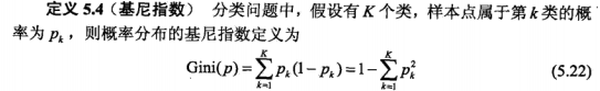
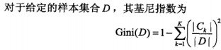
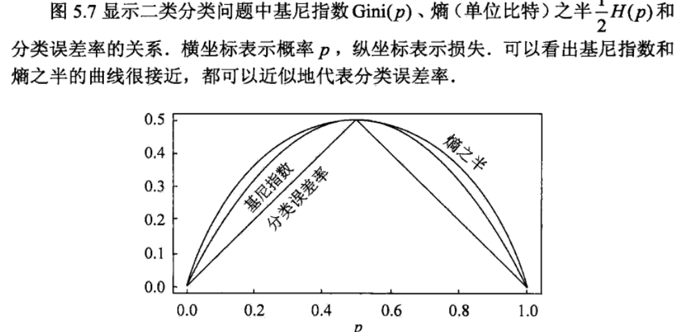
4) 基尼指数（gini index）

这里写图片描述

3）决策树的生成

构建决策树的违代码如下：

这里写图片描述

ID3算法可以参考c4.5 算法，直至（3）步使用信息增益而不是信息增益比！

对于决策树的剪枝，我们在下个单元讲述，先看一下CART算法！
在详细介绍CART方法之前，我们先说明CART方法和ID3 C4.5 的差异！
关键点一：

CART方法会假设决策树是二叉树，内部特征会取值是或者否，左边分支取值是，右边取值否。决策树递归的二分每个特征。

关键点二：

终止条件：直观的情况，当节点包含的数据记录都属于同一个类别时就可以终止分裂了。这只是一个特例，更一般的情况我们计算χ2值来判断分类条件和类别的相关程度，当χ2很小时说明分类条件和类别是独立的，即按照该分类条件进行分类是没有道理的，此时节点停止分裂。还有一种方式就是，如果某一分支覆盖的样本的个数如果小于一个阈值，那么也可产生叶子节点，从而终止Tree-Growth。

关键点三：

剪枝:在CART过程中第二个关键的思想是用独立的验证数据集对训练集生长的树进行剪枝。

CART 分类树：
这里写图片描述

CART回归树：

3.1决策树的编程实现

from math import log
import operator

def createDataSet():              #测试数据集
    dataSet = [[1, 1, 'yes'],
               [1, 1, 'yes'],
               [1, 0, 'no'],
               [0, 1, 'no'],
               [0, 1, 'no']]
    labels = ['no surfacing','flippers']
    #change to discrete values
    return dataSet, labels

def calcShannonEnt(dataSet):     #计算香农商
    numEntries = len(dataSet)
    labelCounts = {}
    for featVec in dataSet: 
        currentLabel = featVec[-1]
        if currentLabel not in labelCounts.keys(): labelCounts[currentLabel] = 0
        labelCounts[currentLabel] += 1
    shannonEnt = 0.0
    for key in labelCounts:
        prob = float(labelCounts[key])/numEntries
        shannonEnt -= prob * log(prob,2) #log base 2
    return shannonEnt
    
def splitDataSet(dataSet, axis, value):         #安给定的特征列，和特征的取值来划分数据集
    retDataSet = []
    for featVec in dataSet:
        if featVec[axis] == value:
            reducedFeatVec = featVec[:axis]     
            reducedFeatVec.extend(featVec[axis+1:])
            retDataSet.append(reducedFeatVec)
    return retDataSet
    
def chooseBestFeatureToSplit(dataSet):
    numFeatures = len(dataSet[0]) - 1      #选出最好的划分特征
    baseEntropy = calcShannonEnt(dataSet)
    bestInfoGain = 0.0; bestFeature = -1
    for i in range(numFeatures):        #iterate over all the features
        featList = [example[i] for example in dataSet]#create a list of all the examples of this feature
        uniqueVals = set(featList)       #get a set of unique values
        newEntropy = 0.0
        for value in uniqueVals:
            subDataSet = splitDataSet(dataSet, i, value)
            prob = len(subDataSet)/float(len(dataSet))
            newEntropy += prob * calcShannonEnt(subDataSet)     
        infoGain = baseEntropy - newEntropy     #calculate the info gain; ie reduction in entropy
        if (infoGain > bestInfoGain):       #compare this to the best gain so far
            bestInfoGain = infoGain         #if better than current best, set to best
            bestFeature = i
    return bestFeature                      #returns an integer

def majorityCnt(classList):               #通过数据集的标签进行投票
    classCount={}
    for vote in classList:
        if vote not in classCount.keys(): classCount[vote] = 0
        classCount[vote] += 1
    sortedClassCount = sorted(classCount.iteritems(), key=operator.itemgetter(1), reverse=True)
    return sortedClassCount[0][0]

def createTree(dataSet,labels):
    classList = [example[-1] for example in dataSet]
    if classList.count(classList[0]) == len(classList): 
        return classList[0]#当数据集中所有的标签都相同时，停止划分，生成叶子节点
    if len(dataSet[0]) == 1: #当没有特征可用的时候，用多数表决的方法生成叶子节点
        return majorityCnt(classList)
    bestFeat = chooseBestFeatureToSplit(dataSet)   #选出最好的特征
    bestFeatLabel = labels[bestFeat]             
    myTree = {bestFeatLabel:{}}                   #用最好特征的对应属性做节点
    del(labels[bestFeat])
    featValues = [example[bestFeat] for example in dataSet]
    uniqueVals = set(featValues)
    for value in uniqueVals:
        subLabels = labels[:]       #找出最好特征的所有可能，来创建分支
        myTree[bestFeatLabel][value] = createTree(splitDataSet(dataSet, bestFeat, value),subLabels)            #在每一个分支上递归的调用生出树的方法
    return myTree                            
    
def classify(inputTree,featLabels,testVec):   #如果到达叶子节点，就返回类标签
                                               #否则就逐层递归
    firstStr = inputTree.keys()[0]
    secondDict = inputTree[firstStr]
    featIndex = featLabels.index(firstStr)
    key = testVec[featIndex]
    valueOfFeat = secondDict[key]
    if isinstance(valueOfFeat, dict): 
        classLabel = classify(valueOfFeat, featLabels, testVec)
    else: classLabel = valueOfFeat
    return classLabel

def storeTree(inputTree,filename):   #存储决策树  调用决策树
    import pickle
    fw = open(filename,'w')
    pickle.dump(inputTree,fw)
    fw.close()
    
def grabTree(filename):  
    import pickle
    fr = open(filename)
    return pickle.load(fr)

画出决策树用来展示：

import matplotlib.pyplot as plt

decisionNode = dict(boxstyle="sawtooth", fc="0.8")
leafNode = dict(boxstyle="round4", fc="0.8")
arrow_args = dict(arrowstyle="<-")

def getNumLeafs(myTree):
    numLeafs = 0
    firstStr = myTree.keys()[0]
    secondDict = myTree[firstStr]
    for key in secondDict.keys():
        if type(secondDict[key]).__name__=='dict':#test to see if the nodes are dictonaires, if not they are leaf nodes
            numLeafs += getNumLeafs(secondDict[key])
        else:   numLeafs +=1
    return numLeafs

def getTreeDepth(myTree):
    maxDepth = 0
    firstStr = myTree.keys()[0]
    secondDict = myTree[firstStr]
    for key in secondDict.keys():
        if type(secondDict[key]).__name__=='dict':#test to see if the nodes are dictonaires, if not they are leaf nodes
            thisDepth = 1 + getTreeDepth(secondDict[key])
        else:   thisDepth = 1
        if thisDepth > maxDepth: maxDepth = thisDepth
    return maxDepth

def plotNode(nodeTxt, centerPt, parentPt, nodeType):
    createPlot.ax1.annotate(nodeTxt, xy=parentPt,  xycoords='axes fraction',
             xytext=centerPt, textcoords='axes fraction',
             va="center", ha="center", bbox=nodeType, arrowprops=arrow_args )
    
def plotMidText(cntrPt, parentPt, txtString):
    xMid = (parentPt[0]-cntrPt[0])/2.0 + cntrPt[0]
    yMid = (parentPt[1]-cntrPt[1])/2.0 + cntrPt[1]
    createPlot.ax1.text(xMid, yMid, txtString, va="center", ha="center", rotation=30)

def plotTree(myTree, parentPt, nodeTxt):#if the first key tells you what feat was split on
    numLeafs = getNumLeafs(myTree)  #this determines the x width of this tree
    depth = getTreeDepth(myTree)
    firstStr = myTree.keys()[0]     #the text label for this node should be this
    cntrPt = (plotTree.xOff + (1.0 + float(numLeafs))/2.0/plotTree.totalW, plotTree.yOff)
    plotMidText(cntrPt, parentPt, nodeTxt)
    plotNode(firstStr, cntrPt, parentPt, decisionNode)
    secondDict = myTree[firstStr]
    plotTree.yOff = plotTree.yOff - 1.0/plotTree.totalD
    for key in secondDict.keys():
        if type(secondDict[key]).__name__=='dict':#test to see if the nodes are dictonaires, if not they are leaf nodes   
            plotTree(secondDict[key],cntrPt,str(key))        #recursion
        else:   #it's a leaf node print the leaf node
            plotTree.xOff = plotTree.xOff + 1.0/plotTree.totalW
            plotNode(secondDict[key], (plotTree.xOff, plotTree.yOff), cntrPt, leafNode)
            plotMidText((plotTree.xOff, plotTree.yOff), cntrPt, str(key))
    plotTree.yOff = plotTree.yOff + 1.0/plotTree.totalD
#if you do get a dictonary you know it's a tree, and the first element will be another dict

def createPlot(inTree):
    fig = plt.figure(1, facecolor='white')
    fig.clf()
    axprops = dict(xticks=[], yticks=[])
    createPlot.ax1 = plt.subplot(111, frameon=False, **axprops)    #no ticks
    #createPlot.ax1 = plt.subplot(111, frameon=False) #ticks for demo puropses 
    plotTree.totalW = float(getNumLeafs(inTree))
    plotTree.totalD = float(getTreeDepth(inTree))
    plotTree.xOff = -0.5/plotTree.totalW; plotTree.yOff = 1.0;
    plotTree(inTree, (0.5,1.0), '')
    plt.show()

#def createPlot():
#    fig = plt.figure(1, facecolor='white')
#    fig.clf()
#    createPlot.ax1 = plt.subplot(111, frameon=False) #ticks for demo puropses 
#    plotNode('a decision node', (0.5, 0.1), (0.1, 0.5), decisionNode)
#    plotNode('a leaf node', (0.8, 0.1), (0.3, 0.8), leafNode)
#    plt.show()

def retrieveTree(i):
    listOfTrees =[{'no surfacing': {0: 'no', 1: {'flippers': {0: 'no', 1: 'yes'}}}},
                  {'no surfacing': {0: 'no', 1: {'flippers': {0: {'head': {0: 'no', 1: 'yes'}}, 1: 'no'}}}}
                  ]
    return listOfTrees[i]

#createPlot(thisTree)

4）决策树的剪枝

ma416539432

关注

0
点赞
踩
1

收藏

觉得还不错? 一键收藏
0
评论
ML机器学习基于树的家族

ML机器学习基于树的家族目录决策树模型与学习特征选择决策树的生成决策树的剪枝 DBGT随机森林 – 1）决策树模型与学习我们来谈一谈机器学习算法中的各种树形算法，包括ID3、C4.5、CART以及基于集成思想的树模型Random Forest和GBDT。本文对各类树形算法的基本思想进行了简单的介绍，重点谈一谈被称为是算法中的“战斗机”，机器学习中的“屠龙刀”的GBDT算法。
复制链接

扫一扫