​【磁场】基于有限元方法 (FEM) 模拟圆柱电容器、平行板电容器、圆形和矩形金属波导、二维散射问题的磁场附matlab代码

 ✅作者简介：热爱科研的Matlab仿真开发者，修心和技术同步精进，代码获取、论文复现及科研仿真合作可私信。

🍎个人主页：Matlab科研工作室

🍊个人信条：格物致知。

更多Matlab完整代码及仿真定制内容点击👇

智能优化算法       神经网络预测       雷达通信       无线传感器        电力系统

信号处理              图像处理               路径规划       元胞自动机        无人机 

物理应用             机器学习

🔥 内容介绍

磁场在电磁学中扮演着至关重要的角色，广泛应用于电力系统、电子设备和生物医学领域。有限元方法 (FEM) 是一种强大的数值技术，可用于模拟复杂几何形状和材料特性的磁场分布。本文将介绍如何使用 FEM 模拟圆柱电容器、平行板电容器、圆形和矩形金属波导以及二维散射问题的磁场。

有限元方法 (FEM)

FEM 是一种基于变分原理的数值方法，用于求解偏微分方程组。它将求解域划分为一系列称为有限元的较小单元，并在每个单元内使用简单的基函数近似未知场变量。通过最小化变分泛函，可以获得近似解。

圆柱电容器

圆柱电容器由两个同轴圆柱形电极组成，中间填充绝缘材料。FEM 模型可以模拟电极之间的电场和磁场分布。电场由高斯定律求解，而磁场则由安培定律求解。

平行板电容器

平行板电容器由两个平行的导电板组成，中间填充绝缘材料。FEM 模型可以模拟电极之间的电场和磁场分布。电场由高斯定律求解，而磁场则由安培定律求解。

圆形金属波导

圆形金属波导是一种圆柱形波导，用于传输电磁波。FEM 模型可以模拟波导内的电磁场分布。电磁场由麦克斯韦方程组求解。

矩形金属波导

矩形金属波导是一种矩形波导，用于传输电磁波。FEM 模型可以模拟波导内的电磁场分布。电磁场由麦克斯韦方程组求解。

二维散射问题

二维散射问题涉及电磁波在障碍物上散射。FEM 模型可以模拟电磁波在障碍物上的散射过程。电磁场由麦克斯韦方程组求解。

模拟步骤

FEM 模拟磁场的步骤如下：

1. 定义几何形状和材料特性。

2. 划分求解域为有限元。

3. 选择合适的基函数。

4. 组装刚度矩阵和载荷向量。

5. 求解线性方程组。

6. 后处理结果，包括磁场分布、磁通量和磁感应强度。

结论

FEM 是一种强大的工具，可用于模拟各种磁场问题。本文介绍了如何使用 FEM 模拟圆柱电容器、平行板电容器、圆形和矩形金属波导以及二维散射问题的磁场。通过遵循本文中概述的步骤，工程师和研究人员可以准确地预测和分析复杂几何形状和材料特性的磁场分布。

📣 部分代码

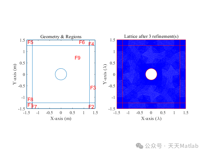
        x(jj,ii +2) = ((-1)^jj) * (w + Cyl_Rad);        y(jj,ii)    = (w + Cyl_Rad + d*(ii-1));        y(jj,ii +2) = (w + Cyl_Rad + d*abs(ii-2));    endendc1 = 3*ones(1,9);c2 = 4*ones(1,9);gd=[c1         1;                     % Creates the matrix for the geometry    c2        xC;                     % Last column consists of the PEC cylinder    x(:,1)'   yC;    x(:,2)' Cyl_Rad;    x(:,4)'    1;    x(:,3)'    1;    y(:,1)'    1;    y(:,2)'    1;    y(:,3)'    1;    y(:,4)'    1];sf = 'R1-R0+R2+R3+R4+R5+R6+R7+R8+R9';                             % setting the formula for the geometryns = char('R1','R2','R3','R4','R5','R6','R7','R8','R9','R0');     % names of the boundariesns = ns';                                                         % converting it to column vector[dl,bt] = decsg(gd,sf,ns);                                        % creates the geometryfigure subplot(1,2,1)pdegplot(dl,'FaceLabels','on');              % plot the resulted geometryaxis equal, axis tightxlabel('X-axis (m)'),ylabel('Y-axis (m)')    % XY-labeltitle('Geometry & Regions'), hold off%% ---------- creates the triangularization ------------------------------refin = 3;                           % choose the number of refinements you want  <---------------------[p,e,t] = initmesh(dl);              % creates the triangularizationfor ii = 1:refin    [p,e,t] = refinemesh(dl,p,e,t);  % denses the triangular latticeendsubplot(1,2,2)pdeplot(p/lambda,e,t);               % plot the geometry with the triagualrizationaxis equal, axis tightxlabel('X-axis (\lambda)'),ylabel('Y-axis (\lambda)')   % XY-labelstitle(['Lattice after ',num2str(refin),' refinement(s)']),hold off​%% Preparations and initializations for the MAIN part Nn      = size(p,2);   % total number of nodesNe      = size(t,2);   % total number of elementsNd      = size(e,2);   % number of edges - ακμέςnode_id = ones(Nn,1);  % to identify if a node is KNOWN or UNKNOWNEi      = zeros(Nn,1); % incident fieldEs      = zeros(Nn,1); % Scattered Field​% Calculte the incident field Ei in the main computational windowfor ie = 1:Ne    n(1:3) = t(1:3,ie);    rg     = t(4,ie);    x(1:3) = p(1,n(1:3));    y(1:3) = p(2,n(1:3));    if rg == 9       % the largerest area is alaways at the bottom line        for ii = 1:3            Ei(n(ii)) = Eo * exp(-1i*k0*(x(ii)));        end    endend​% Boundary conditionsfor ii = 1:Nd    if (e(6,ii) == 0 || e(7,ii) == 0 )        for jj = 1:2            % the following IF checks if we are on the boundary of the PEC cylinder or            % the total window            if ( abs( p(1,e(jj,ii)) ) < (Cyl_Rad + w )  &&  abs( p(2,e(jj,ii)) ) < (Cyl_Rad + w) )                node_id(e(jj,ii)) = 0;                % defines the node as known                Es(e(jj,ii))      = - Ei(e(jj,ii));   % defines the Dirichlet condition on the PEC cylider            end        end    endend% Re-enumerating the UNKNOWNS !counter = 0;index   = zeros(Nn,1);for ii = 1:Nn    if node_id(ii) == 1        counter = counter + 1;        index(ii) = counter;     % index for the unknowns    endend%% Main - Kernel Calculation of Stiffness and Mass Matrices ------------Nf  = nnz(node_id);                 % number of uknown variablesSff = spalloc(Nf,Nf,7*Nf);          % initialization of the large Stiff Matrix for system Solutions Sff*X = BB   = zeros(Nf,1);Aet = spalloc(Nf,Nf,7*Nf);​​muxx(1) = mu0;         % computational window, the area where field is beingmuyy(1) = mu0;         % calculatedezz(1)  = e_r*e0;%muxx(2) = mu0*llx(1);  % left and right X regions with PMLmuyy(2) = mu0*llx(2);ezz(2)  = e0* llx(3);%muxx(3) = mu0*lly(1);  % top and bottom Y regions with PMLmuyy(3) = mu0*lly(2);ezz(3)  = e0* lly(3);%muxx(4) = mu0*llxy(1); % overlapping xy regions with PMLmuyy(4) = mu0*llxy(2);ezz(4)  = e0* llxy(3);​% -------- MAIN LOOP ------------------------------------------------------S  = zeros(3,3);Te = zeros(3,3);T  = (1/12) * ones(3);                  % local Mass Matrix is standard !T  = T - (1/12)*eye(3) + (1/6)*eye(3);  % Te = Ae* [1/6    1/12   1/12;%                                                   1/12   1/6    1/12;%                                                   1/12   1/12    1/6 ];ticfor ie = 1:Ne    n(1:3) = t(1:3,ie);            % n(1:3) are the nodes of every elemnet    rg     = t(4,ie);              % rg is the region of the element (subdomain number)    x(1:3) = p(1,n(1:3));          % stores the x-coordinate    y(1:3) = p(2,n(1:3));          % stores the y-coordinate    De     = det([1 x(1) y(1);1 x(2) y(2);1 x(3) y(3)]);  % determinant    Ae     = abs(De/2);            % element area        b(1) = ( y(2) -y(3) ) / De ;    % Coefficients for linea    b(2) = ( y(3) -y(1) ) / De ;    % triangular finite elements. For more    b(3) = ( y(1) -y(2) ) / De ;    % information on these equations read Tsimboukis'    c(1) = ( x(3) -x(2) ) / De ;    % complementary books "Notes on Computational Electromagnetics" pages 83-95    c(2) = ( x(1) -x(3) ) / De ;    % and "Energy Methods for E/M Fields" pages 287-308    c(3) = ( x(2) -x(1) ) / De ;    % Calculate the Se & Te for each region Correctly!!    if rg == 9        id = 1;    elseif ( rg == 1 || rg == 2 || rg == 4 || rg == 5 )  % overlapping XY PML region        id = 4;    elseif ( rg == 6 || rg == 7 )                        % Y PML region        id = 3;    else%if ( rg == 3 || rg == 8 )                       % X PML region        id = 2;    end        %     S = zeros(3,3);    Te = ezz(id)*Ae * T;                     % Calculates Local Mass Matrix    for ii = 1:3        for jj = 1:3                         % Calculates Local Stiffness Matrix            S(ii,jj) = (1/muyy(id) * b(ii)*b(jj) + 1/muxx(id) * c(ii)*c(jj))*Ae;            if ( node_id(n(ii)) ~= 0 )                if ( node_id(n(jj)) ~= 0 )                    Aet(index(n(ii)) , index(n(jj))) = ...                        Aet(index(n(ii)) , index(n(jj))) + S(ii,jj) - (omega^2)*Te(ii,jj);                else                    B(index(n(ii))) = B(index(n(ii))) - ( S(ii,jj) - (omega^2)*Te(ii,jj))*Es(n(jj) );                end                            end        end            endendtocX = Aet\B;                           % direct solverfor i =1:Nn    if index(i) ~= 0                 % completing the result vector after the system solution        Es(i) = X(index(i)) ;        % by creating a total vector including the boundaries    endendE = Es+Ei ;                          % total Electric Field = Scattered and Incident%%  FEM plots figuresubplot(2,2,1)                 % plot the real part of the total fieldpdeplot(p/lambda,e,t,'XYdata',real(E),'Contour','off')axis equal; axis tight;colormap(jet);hcb = colorbar;hcb.Label.String = 'V/m';xlim([x_min x_max]/lambda), ylim([y_min y_max]/lambda)  % XY-limitsxlabel('X-axis (\lambda)'), ylabel('Y-axis (\lambda)')  % XY-labeltitle('Real\{E\}')​subplot(2,2,2)                % plot the imaginary part of the total fieldpdeplot(p/lambda,e,t,'XYdata',imag(E),'Contour','off')axis equal; axis tight;colormap(jet);hcb = colorbar;hcb.Label.String = 'V/m';xlim([x_min x_max]/lambda), ylim([y_min y_max]/lambda)  % XY-limitsxlabel('X-axis (\lambda)'), ylabel('Y-axis (\lambda)')  % XY-labeltitle('Imag\{E\}')​subplot(2,2,3:4)              % plot the magnitude of the total fieldpdeplot(p/lambda,e,t,'XYdata',abs(E),'Contour','off')axis equal; axis tight;colormap(jet);hcb = colorbar;hcb.Label.String = 'V/m';xlim([x_min x_max]/lambda), ylim([y_min y_max]/lambda)  % XY-limitsxlabel('X-axis (\lambda)'), ylabel('Y-axis (\lambda)')  % XY-labeltitle('|E|')hold offsg = sgtitle({'Total Electric Field   E = E_i + E_s'});sg.FontName    = 'Times';

⛳️ 运行结果

🔗 参考文献

[1] 王洋,王昕.基于J—A模型磁滞回线仿真及有效性研究[J].农业科技与装备, 2011.DOI:CNKI:SUN:NYJD.0.2011-10-023.

[2] 李晓飞,刘连光.基于J-A模型磁滞回线仿真及有效性研究[C]//华北电力大学研究生学术交流年会.华北电力大学, 2007.

🎈 部分理论引用网络文献，若有侵权联系博主删除

🎁  关注我领取海量matlab电子书和数学建模资料

👇  私信完整代码和数据获取及论文数模仿真定制

1 各类智能优化算法改进及应用

生产调度、经济调度、装配线调度、充电优化、车间调度、发车优化、水库调度、三维装箱、物流选址、货位优化、公交排班优化、充电桩布局优化、车间布局优化、集装箱船配载优化、水泵组合优化、解医疗资源分配优化、设施布局优化、可视域基站和无人机选址优化、背包问题、 风电场布局、时隙分配优化、 最佳分布式发电单元分配、多阶段管道维修、 工厂-中心-需求点三级选址问题、 应急生活物质配送中心选址、 基站选址、 道路灯柱布置、 枢纽节点部署、 输电线路台风监测装置、 集装箱船配载优化、 机组优化、 投资优化组合、云服务器组合优化、 天线线性阵列分布优化

2 机器学习和深度学习方面

2.1 bp时序、回归预测和分类

2.2 ENS声神经网络时序、回归预测和分类

2.3 SVM/CNN-SVM/LSSVM/RVM支持向量机系列时序、回归预测和分类

2.4 CNN/TCN卷积神经网络系列时序、回归预测和分类

2.5 ELM/KELM/RELM/DELM极限学习机系列时序、回归预测和分类

2.6 GRU/Bi-GRU/CNN-GRU/CNN-BiGRU门控神经网络时序、回归预测和分类

2.7 ELMAN递归神经网络时序、回归\预测和分类

2.8 LSTM/BiLSTM/CNN-LSTM/CNN-BiLSTM/长短记忆神经网络系列时序、回归预测和分类

2.9 RBF径向基神经网络时序、回归预测和分类

2.10 DBN深度置信网络时序、回归预测和分类

2.11 FNN模糊神经网络时序、回归预测

2.12 RF随机森林时序、回归预测和分类

2.13 BLS宽度学习时序、回归预测和分类

2.14 PNN脉冲神经网络分类

2.15 模糊小波神经网络预测和分类

2.16 时序、回归预测和分类

2.17 时序、回归预测预测和分类

2.18 XGBOOST集成学习时序、回归预测预测和分类

方向涵盖风电预测、光伏预测、电池寿命预测、辐射源识别、交通流预测、负荷预测、股价预测、PM2.5浓度预测、电池健康状态预测、用电量预测、水体光学参数反演、NLOS信号识别、地铁停车精准预测、变压器故障诊断

2.图像处理方面

图像识别、图像分割、图像检测、图像隐藏、图像配准、图像拼接、图像融合、图像增强、图像压缩感知

3 路径规划方面

旅行商问题（TSP）、车辆路径问题（VRP、MVRP、CVRP、VRPTW等）、无人机三维路径规划、无人机协同、无人机编队、机器人路径规划、栅格地图路径规划、多式联运运输问题、 充电车辆路径规划（EVRP）、 双层车辆路径规划（2E-VRP）、 油电混合车辆路径规划、 船舶航迹规划、 全路径规划规划、 仓储巡逻

4 无人机应用方面

无人机路径规划、无人机控制、无人机编队、无人机协同、无人机任务分配、无人机安全通信轨迹在线优化、车辆协同无人机路径规划

5 无线传感器定位及布局方面

传感器部署优化、通信协议优化、路由优化、目标定位优化、Dv-Hop定位优化、Leach协议优化、WSN覆盖优化、组播优化、RSSI定位优化

6 信号处理方面

信号识别、信号加密、信号去噪、信号增强、雷达信号处理、信号水印嵌入提取、肌电信号、脑电信号、信号配时优化

7 电力系统方面

微电网优化、无功优化、配电网重构、储能配置、有序充电

8 元胞自动机方面

交通流 人群疏散 病毒扩散 晶体生长 金属腐蚀

9 雷达方面

卡尔曼滤波跟踪、航迹关联、航迹融合