Fluxnet2015 数据集学习

FLUXNET 2015版本的FULLSET数据产品包括数据产品的所有变量，包括所有质量和不确定性变量，以及来自数据处理管道中中间数据处理步骤的一些选定变量。

ERAI Data Product

辅助数据产品，包含使用ERA临时再分析数据产品（详细信息请参阅有关数据处理管道的文件）缩小规模的微气象变量（与现场测量变量相关）的完整记录（1989-2014年）。

AUXMETEO Data Product

辅助数据产品，包含使用ERA临时再分析数据产品缩小微气象变量的结果。此文件中的变量与缩减中使用的每个数据变量的线性回归和误差/相关性估计相关。

Variables (see list below): TA, PA, VPD, WS, P, SW_IN, LW_IN, LW_IN_JSB

Parameters:

Parameters:

• ERA_SLOPE: slope of linear regression线性回归的斜率
• ERA_INTERCEPT: intercept point of linear regression线性回归的截取点
• ERA_RMSE: root mean square error between site data and downscaled data站点数据和降尺度数据之间的均方误差
• ERA_CORRELATION: correlation coefficient of linear fit (R-Squared == ERA_CORRELATION * ERA_CORRELATION)

• AUXNEE Data Product

• 包含NEE处理（主要与USTAR过滤相关）以及RECO和GPP生成产生的变量的辅助数据产品。本产品中的变量包括USTAR过滤方法执行的成功/失败、应用于不同版本变量的USTAR阈值以及具有最佳模型效率结果的百分位/阈值对。

• Variables:

• USTAR_MP_METHOD: Moving Point Test USTAR threshold method run
• USTAR_CP_METHOD: Change Point Detection USTAR threshold method run
• NEE_USTAR50_[UT]: NEE using 50-percentile ofUSTAR thresholds from bootstrapping at USTAR filtering step using method UT (CUT, VUT)
• NEE_[UT]_REF: Reference NEE, using model efficiency approach, using method UT (CUT, VUT)
• [PROD]_[ALG]_[UT]_REF: Reference product PROD (RECO or GPP), using model efficiency approach, using algorithm ALG(NT, DT) for partitioning and method UT (CUT, VUT)
• SUCCESS_RUN: 1 if run of method (USTAR_MP_METHOD or USTAR_CP_METHOD) was successful, 0 otherwise
• USTAR_PERCENTILE: percentile of USTAR thresholds from bootstrapping at USTAR filtering step
• USTAR_THRESHOLD: USTAR threshold value corresponding to USTAR_PERCENTILE
• [RR]_USTAR_PERCENTILE: percentile of USTAR thresholds from bootstrapping at USTAR filtering step at resolution RR (HH, DD, WW, MM, YY)
• [RR]_USTAR_THRESHOLD: USTAR threshold value corresponding to USTAR_PERCENTILE at resolution RR (HH, DD, WW, MM, YY)

Variables in the FULLSET Data Product (all variables)

TA 温度 MDS应该是一种数据质量控制方法 ERA是用ERA再分析的数据  _QC质量控制指数

SW短波辐射 LW长波辐射 VPD水汽压差（这是和饱和水气压作差吗？）

DD 半小时平均  WW-YY日数据平均 

_F的一般是经过两种资料结合的一个数据

TA_F_MDS

deg C

Air temperature, gapfilled using MDS method

TA_F_MDS_NIGHT

deg C

Average nighttime TA_F_MDS

TA_F_MDS_NIGHT_SD

deg C

Standard deviation for TA_F_MDS_NIGHT

TA_F_MDS_DAY

deg C

Average daytime TA_F_MDS

TA_F_MDS_DAY_SD

deg C

Standard deviation for TA_F_MDS_DAY

TA_ERA

deg C

Air temperature, downscaled from ERA, linearly regressed using measured only site data

TA_ERA_NIGHT

deg C

Average nighttime TA_ERA

TA_ERA_NIGHT_SD

deg C

Standard deviation for TA_ERA_NIGHT

TA_ERA_DAY

deg C

Average daytime TA_ERA

TA_ERA_DAY_SD

deg C

Standard deviation for TA_ERA_DAY

TA_F

deg C

Air temperature, consolidated from TA_F_MDS and TA_ERA

TA_F_NIGHT

deg C

Average nighttime TA_F

TA_F_NIGHT_SD

deg C

Standard deviation for TA_F_NIGHT

TA_F_DAY

deg C

Average daytime TA_F

TA_F_DAY_SD

deg C

Standard deviation for TA_F_DAY

SW_IN_POT

W m-2

Shortwave radiation, incoming, potential (top of atmosphere)

SW_IN_F_MDS

W m-2

Shortwave radiation, incoming, gapfilled using MDS (negative values set to zero, e.g., negative values from instrumentation noise)

SW_IN_ERA

W m-2

Shortwave radiation, incoming, downscaled from ERA, linearly regressed using measured only site data (negative values set to zero)

SW_IN_F

W m-2

Shortwave radiation, incoming consolidated from SW_IN_F_MDS and SW_IN_ERA (negative values set to zero)

LW_IN_F_MDS

W m-2

Longwave radiation, incoming, gapfilled using MDS

LW_IN_ERA

W m-2

Longwave radiation, incoming, downscaled from ERA, linearly regressed using measured only site data

LW_IN_F

W m-2

Longwave radiation, incoming, consolidated from LW_IN_F_MDS and LW_IN_ERA

LW_IN_JSB

W m-2

Longwave radiation, incoming, calculated from TA_F_MDS, SW_IN_F_MDS, VPD_F_MDS and SW_IN_POT using the JSBACH algorithm (Sonke Zaehle)

LW_IN_JSB_ERA

W m-2

Longwave radiation, incoming, downscaled from ERA, linearly regressed using site level LW_IN_JSB calculated from measured only drivers

LW_IN_JSB_F

W m-2

Longwave radiation, incoming, consolidated from LW_IN_JSB and LW_IN_JSB_ERA

VPD_F_MDS

hPa

Vapor Pressure Deficit, gapfilled using MDS蒸汽压差

VPD_ERA

hPa

Vapor Pressure Deficit, downscaled from ERA, linearly regressed using measured only site data

VPD_F

hPa

Vapor Pressure Deficit consolidated from VPD_F_MDS and VPD_ERA

PA

kPa

Atmospheric pressure

气压的单位是KPa ，注意！

P

mm

Precipitation

WS

m s-1

Wind speed风速

WD

Decimal degrees十进制度

Wind direction风向

RH

%

Relative humidity, range 0-100

USTAR

m s-1

Friction velocity

NETRAD

W m-2

Net radiation

PPFD_IN

µmolPhoton m-2 s-1

Photosynthetic photon flux density, incoming光合光子通量密度？入射

PPFD_DIF

µmolPhoton m-2 s-1

Photosynthetic photon flux density, diffuse incoming光合光子通量密度，入射

PPFD_OUT

µmolPhoton m-2 s-1

Photosynthetic photon flux density, outgoing光合光子通量密度，出射

SW_DIF

W m-2

Shortwave radiation, diffuse incoming

SW_OUT

W m-2

Shortwave radiation, outgoing

LW_OUT

W m-2

Longwave radiation, outgoing

CO2_F_MDS

W m-2

CO2 mole fraction, gapfilled with MDS

TS_F_MDS_#

Soil temperature, gapfilled with MDS (numeric index “#” increases with the depth, 1 is shallowest)

TS 土壤温度 #代表层数，1是最浅层

ENERGY PROCESSING

G_F_MDS

W m-2

Soil heat flux

LE_F_MDS

W m-2

Latent heat flux, gapfilled using MDS method

LE_CORR

W m-2

Latent heat flux, corrected LE_F_MDS by energy balance closure correction factor

H_F_MDS

W m-2

Sensible heat flux, gapfilled using MDS method

H_CORR

W m-2

Sensible heat flux, corrected H_F_MDS by energy balance closure correction factor

H_CORR_25

W m-2

Sensible heat flux, corrected H_F_MDS by energy balance closure correction factor, 25th percentile

H_CORR_75

W m-2

Sensible heat flux, corrected H_F_MDS by energy balance closure correction factor, 75th percentile

H_RANDUNC

W m-2

Random uncertainty of H, from measured only data

NET ECOSYSTEM EXCHANGE

NIGHT		Flag indicating nighttime interval based on SW_IN_POT
HH	nondimensional	0 = daytime, 1 = nighttime

NIGHT_D

Number of half hours classified as nighttime in the period, i.e., when SW_IN_POT is 0

DAY_D

Number of half hours classified as daytime in the period, i.e., when SW_IN_POT is greater than 0

NEE_CUT_REF		Net Ecosystem Exchange, using Constant Ustar Threshold (CUT) across years, reference selected on the basis of the model efficiency (MEF). The MEF analysis is repeated for each time aggregation
HH	umolCO2 m-2 s-1
DD	gC m-2 d-1	calculated from half-hourly data
WW-MM	gC m-2 d-1	average from daily data
YY	gC m-2 y-1	sum from daily data

NEE_VUT_REF

Net Ecosystem Exchange, using Variable Ustar Threshold (VUT) for each year, reference selected on the basis of the model efficiency (MEF). The MEF analysis is repeated for each time aggregation净生态系统交换，使用跨年度的恒定Ustar阈值（CUT），基于模型效率（MEF）选择参考。MEF分析对每个时间聚合重复进行。？这个关于生态的我不太懂了，之后如果相关研究我再看这个，以下省略相关变量

GPP  Gross Primary Production  总初级生产力

RECO  Ecosystem Respiration  生态系统呼吸

FLUXNET2015文章翻译

原文链接The FLUXNET2015 dataset and the ONEFlux processing pipeline for eddy covariance data | Scientific Data

摘要

FLUXNET2015 数据集提供了全球 212 个站点的生态系统规模的二氧化碳、水和能量交换数据，以及其他气象和生物测量数据（涵盖超过 1500 个站年，截至 2014 年）。这些独立管理和运营的站点自愿贡献数据以创建全球数据集。数据经过质量控制和统一方法处理，以提高各站点之间的一致性和可比性。该数据集已被用于多个应用中，包括生态生理学研究、遥感研究以及生态系统和地球系统模型的开发。FLUXNET2015 包括衍生数据产品，如填补缺口的时间序列、生态系统呼吸和光合作用吸收估计、不确定性估计以及关于测量的元数据，这些数据在本文中首次呈现。此外，这 206 个站点首次以创意共享（CC-BY 4.0）许可证进行分发。本文详细介绍了这一增强数据集及其处理方法，这些方法现在以开源代码的形式提供，使数据集更加可访问、透明和可重复。

背景和总结

过去三十多年来，涡旋协方差技术¹被用于全球范围内的测量站，研究和确定生态系统和气候系统的功能和轨迹，通过这一技术可以测量陆地与大气之间的温室气体和能量交换。该技术能够以高时间分辨率和生态系统水平对这些通量进行非破坏性测量，使其成为一种独特的工具。基于对垂直风速和标量（CO₂、H₂O、温度等）的高频（10–20 Hz）测量，该技术提供了对标量在测量点周围几百米范围内源区足迹面积的净交换量估计。

首先运营的几处一致性测量站投入使用后，欧洲²和美国³⁴陆续建立了区域站点网络，此后其他大陆也相继推出了类似计划⁵⁶⁷。这些网络使得涡旋协方差数据的应用超越了单一站点或生态系统，实现了跨站点比较和区域到全球范围内的研究⁸⁻¹⁵。这些区域网络发展成为长期的研究基础设施或监测活动，如ICOS、AmeriFlux、NEON、AsiaFlux、ChinaFLUX和TERN-OzFlux。

FLUXNET作为一个全球网络的网络¹⁶⁻¹⁸诞生，是区域网络之间的一项联合努力，旨在协调和提高数据收集标准化水平。它使得全球涡旋协方差数据集的创建成为可能。第一套包含填补缺口的全球FLUXNET数据集于2000年发布，名为Marconi数据集¹⁹，其包含97个站年数据，并引入了光合作用和呼吸等分区通量等衍生数据，随后2007年发布了LaThuile数据集²⁰，包含965个站年数据，最后于2015年发布了FLUXNET2015数据集¹⁸²¹（以下简称FLUXNET2015），包含1532个站年数据。每个数据集包含的站点和年数受到两个主要因素的限制：数据政策和数据质量。愿意在所选数据政策下共享数据是FLUXNET2015很可能仅包含全球现有站点的10–20%的主要原因——现有站点的总数仍然未知。其次是数据处理管道和质量控制的演进，导致在数据中识别出新的问题，如果及时未能解决，这些数据将被排除在外。LaThuile数据集的数据政策更为严格，并在某些情况下发现了先前未发现的数据问题，导致FLUXNET2015包含的站点数量较少。

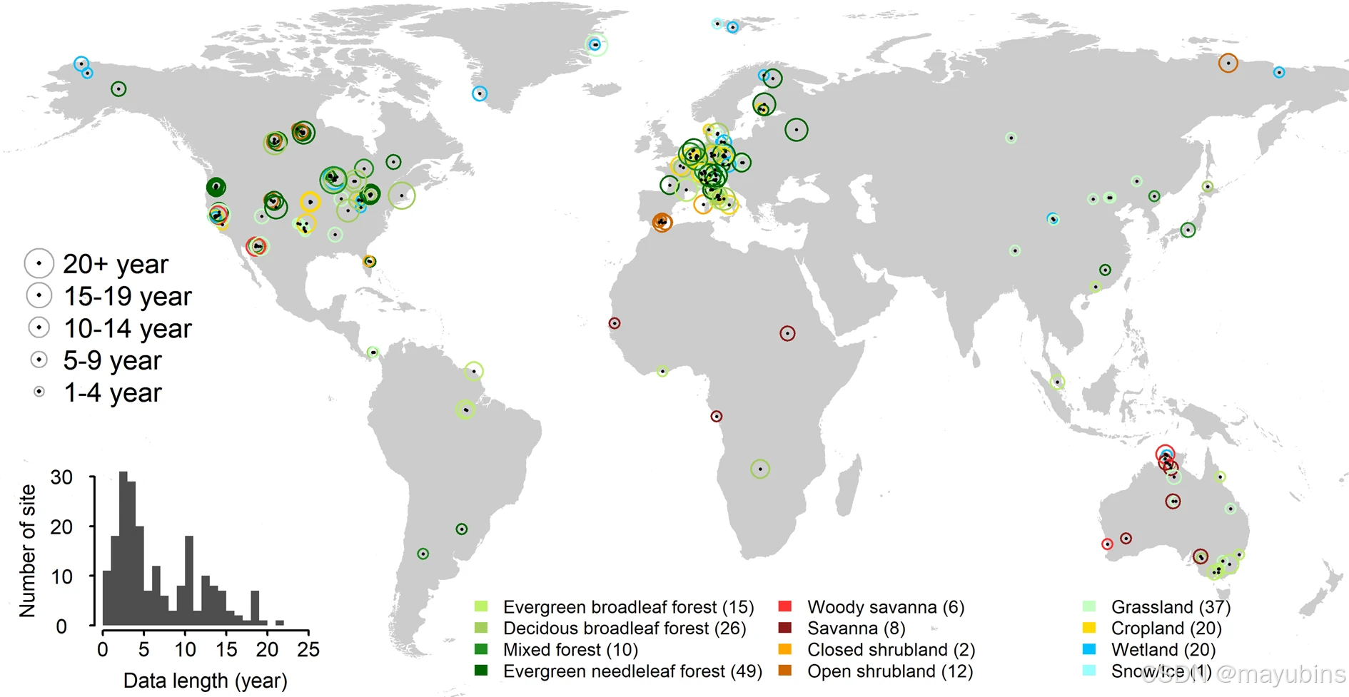
FLUXNET2015首次包含了记录时间超过二十年的站点数据（图1）。该数据集通过许多区域网络的合作创建，数据准备工作在站点、区域网络和全球网络水平上进行。数据准备活动的全球协调和数据处理由AmeriFlux管理项目（AMP）、欧洲生态系统通量数据库和ICOS生态系统主题中心（ICOS-ETC）团队负责。该团队负责编码工作、质量检查和数据处理管道的执行。这些共同努力导致了一个标准化的数据集，标准化的方面包括（1）数据产品本身，（2）数据分发格式，以及（3）各站点的数据质量。这些数据集在全球合成和建模活动中的广泛应用凸显了其价值。然而，数据的异质性——主要由数据收集、通量计算和提交前数据整理的差异引起——突显了数据不确定性估计和统一数据质量评估的必要性。

本文包含的206个塔站地图，这些塔站选自于FLUXNET2015数据集2020年2月发布的212个站点。圆圈大小表示数据记录的长度，圆圈颜色代表生态系统类型，依据国际地圈-生物圈计划（IGBP）定义。重叠时，位置略微偏移以提高可读性。括号内的数字表示每个IGBP组的站点数量。插图显示数据记录长度的分布。见补充图SM4可获取澳大利亚、欧洲和北美洲的continental尺度地图。

该数据处理管道采用了成熟且发表的方法，同时也实施了新的代码，并从社区提供的实施中调整了代码。该管道的主要产品包括：(1)全面的数据质量控制检查；(2)计算一系列摩擦速度阈值，用于过滤低湍流时期，从而能够同时估算此次过滤引起的不确定性和随机不确定性；(3)对气象和通量测量进行缺测填补，其中包括使用降尺度再分析数据产品来填补气象变量的长时间缺失；(4)使用三种不同的方法将二氧化碳通量划分为呼吸和光合作用（总初级生产力）组件；以及(5)计算能量通量的校正因子，以估算该站点能量收支闭合的偏差。本管道的两个特点是摩擦速度阈值的范围以及用于划分二氧化碳通量的多种方法。这两种特点都支持对处理步骤本身引入的不确定性进行更全面评估。我们对该管道的实现以名为ONEFlux（开放网络启用通量处理管道）的开源代码包的形式公开。 本文的目标是描述FLUXNET2015及其附加产品，介绍该处理管道的详细信息，并记录生成该数据集所采用的方法。通过此举，FLUXNET数据的最终用户社区将获得必要的技术和实践知识，以充分发挥FLUXNET数据的潜力，包括FLUXNET2015版本发布的数据，以及自发布后提交至网络的数据。

数据处理方法

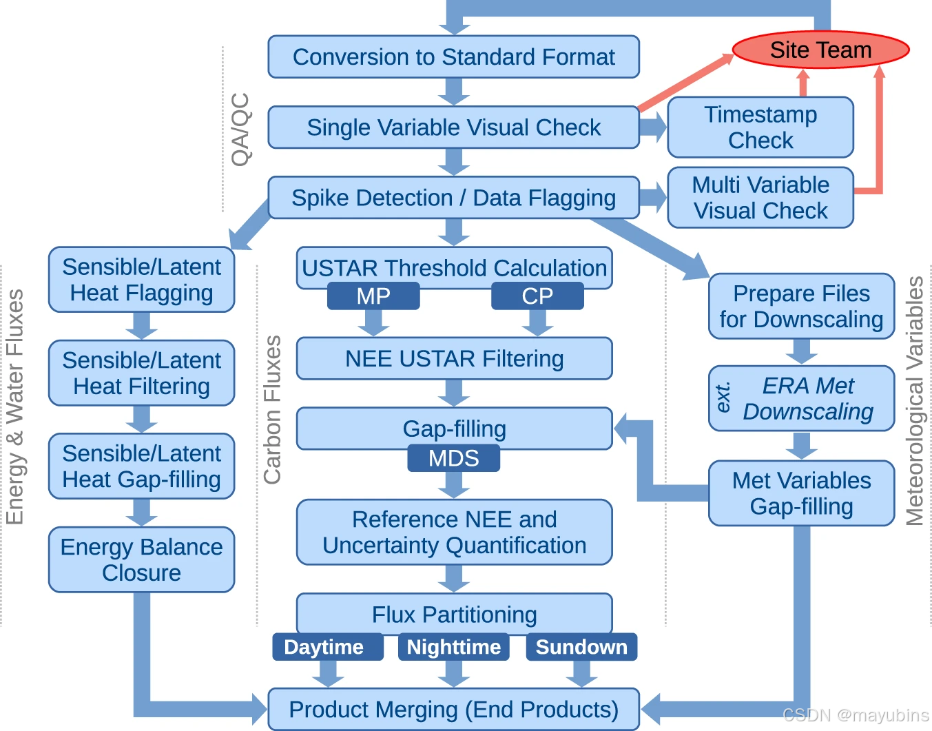
FLUXNET2015中包含的数据是由各站点团队提交的，涵盖了通量、气象、环境和土壤时间序列数据，且这些数据的时间分辨率为半小时或一小时。提交的数据经过了统一的数据质量控制流程，数据问题在与站点团队协商后得到解决。随后，数据通过本节所述的处理管道（图2）进行处理。生成的数据产品通过FLUXNET-Fluxdata网页门户23进行分发，通过注册所有请求并提供使用者的详细信息来追踪数据集的使用情况。这些信息对于更好地理解用户需求以及数据集的影响至关重要。

FLUXNET2015数据处理步骤的逻辑（文本中不同步骤的详细内容及缩写词的含义）。

数据来源
首级数据处理由各站点团队完成，包括从高频风和浓度测量计算半小时或小时湍流通量、对时间分辨率较短的气象变量进行平均，以及站点团队自身的质量控制程序。提交的通量数据需分开为湍流通量和储存通量（总通量的组成部分）单独提交，并未对低湍流条件进行缺测填补或过滤——详见Aubinet等人24的研究。实施了控制检查以确保如此处理，并检测其他不一致性问题以要求站点团队解决，例如时间戳的一致性、相关变量间的连贯性等25。从这些数据出发，我们对所有其余处理步骤（从过滤到缺测填补和划分）应用了相同的方法集，提高了统一性，并允许量化处理引起的不确定性。数据的协调统一——尤其是数据质量的统一——在创建数据集时是重中之重，因此需要与站点团队进行大量互动。数据通过区域网络提交，并将网络提供的格式转换为标准化输入用于处理。这一FLUXNET数据集促成了一个新的跨网络规范，用于标准站点数据和元数据提交格式，该规范现已被不同区域网络采用。

数据处理流水线概述
数据处理流水线（图2）分为四个主要处理模块。第一个模块是我们团队对所有站点数据应用的数据质量保证与质量控制（QA/QC）活动。这一部分结合了自动化程序和手动检查，适用于所有提交的变量。接下来的三个模块均属于自动化处理流水线，分别为每个站点单独执行：能量与水分量处理模块涵盖了感热和潜热变量；碳通量处理模块处理二氧化碳通量变量，如净生态系统交换（NEE）；气象变量处理模块处理所有气象测量，这些测量也用于通量和其他产品的处理。在每个处理步骤中，强制执行一套自动化的前置和后置条件，确保每个步骤的输入和输出符合预期行为。最后一步涉及合并前一步生成的所有产品，并添加从日到年的时间聚合，最多变量的数据集和相关质量标志。该步骤执行了所有变量的一致性自动检查，并创建了所有提交和生成的数据产品的最终文件，以便分发。补充图SM2展示了处理流水线中按代码序列组织的总体步骤，该流水线在ONEFlux包22中公开。所有步骤均已在共享代码中实现，唯独日落划分法（见实施方法部分详细内容）。

结果合集
采用多种方法处理同一处理步骤（例如，计算USTAR阈值的两种方法，或用于划分二氧化碳通量的两种或三种方法，详见本节下文）是由于文献中存在不同的方法，这些方法使用了不同的假设并可能产生不同的结果26,27。一方面，这种方法的不统一可能对合成研究构成问题。另一方面，采用单一方法可能导致偏差，并低估方法学中的不确定性。我们采用的方法同时采用了多种方法，允许创建一个合集，帮助评估不确定性，并评估单个方法对站点条件的适用性。

数据质量保证与控制
在生成衍生数据产品（此后称为后处理）的处理之前，各站点的数据需通过Pastorello等人25提出的QA/QC检查。数据集中的所有变量均进行了检查，而关键变量则接受了进一步的审查。这些额外的检查针对的是处理至关重要的变量，例如通量变量、用于缺测填补的气象变量，以及不确定性估算程序使用的变量。对于关键变量存在待解决问题的站点，处理将不继续进行。

后处理的关键元数据变量：

站点的FluxID，形式为CC-SSS（两个字符的国家代码，三个字符的国家内站点标识符）–例如，US-Ha1

站点的经纬度，以WGS 84十进制格式表示，分辨率至少为四位小数–例如，42.5378/−72.1715

站点的时区（时间序列，如果时区发生变化；时间戳均为当地标准时间，无夏令时）–例如，UTC-5

气体分析仪的高度–例如，30.0 米

后处理的关键数据变量，平均或积分为30或60分钟（*表示必填）：

*CO2 (µmolCO2 mol−1)：湿空气中的二氧化碳（CO2）摩尔分数

*FC (µmolCO2 m−2 s−1)：二氧化碳（CO2）湍流通量（不包含储存组件）

*SC (µmolCO2 m−2 s−1)：使用垂直剖面系统测量的二氧化碳（CO2）储存通量，若塔高短于3米可选

*H (W m−2)：感热湍流通量，不含储存校正

*LE (W m−2)：潜热湍流通量，不含储存校正

*WS (m s−1)：水平风速

*USTAR (m s−1)：阻力速度

*TA (deg C)：空气温度

*RH (%): 相对湿度（范围0–100%）

*PA (kPa): 大气压

G (W m−2): 地面热流，不强制要求，但需要用于能量平衡闭合计算

NETRAD (W m−2): 网辐射，不强制要求，但需要用于能量平衡闭合计算

*SW_IN (W m−2): 入来短波辐射

SW_IN_POT (W m−2): 入来短波辐射的潜在值（大气顶部理论最大辐射），基于站点坐标计算22

PPFD_IN (µmolPhotons m−2 s−1): 入来光合作用光子通量密度

P (mm): 每30或60分钟的降水总量

LW_IN (W m−2): 入来（下行）长波辐射

SWC (%): 土壤含水量（体积含水量），范围0–100%

TS (deg C): 土壤温度

文件格式标准化
为了处理数百个站点的数据，我们需要一致的文件格式来支持输入数据和元数据。这导致了多网络协议的达成，并为数据和元数据向区域网络贡献创建了格式28,29。这些格式已被欧洲和美洲的网络以及一些仪器制造商采用，并被其他区域网络考虑中。此外，为了直接格式转换，实施了自动化提取和转换工具，以便处理旧格式数据。

数据QA/QC步骤
在处理开始前检查了数据质量。如果网络级数据团队无法解决识别出的问题，站点团队将被要求提出处理方案或发送解决质量问题的新数据版本。主要的数据QA/QC步骤包括：单变量检查、多变量检查、专用检查和自动检查。单变量检查逐个查看一变量在时间序列中的模式，长期和短期趋势及其他问题。多变量检查查看相关变量之间的关系（例如，不同辐射变量），以识别存在不一致的时间段。专用检查测试生态和气象数据中常见的问题，如时间戳偏移或传感器退化。在此阶段，使用纬度/经度坐标和时间22，还计算了顶部大气潜在辐射（SW_IN_POT）的时间序列。这三类检查在Pastorello等人25的研究中详细说明。自动检查应用了Papale等人30的反脉冲程序，并对每个变量应用一套范围控制。此最后一步创建了一系列标志，这些标志与站点管理人员讨论以更正和重新提交，然后用于后续步骤的数据过滤。

气象数据产品
对气象数据的主要处理是通过两种独立方法进行缺测填补：边际分布抽样31（MDS）和ERA-Interim32。使用MDS方法填补缺测的数据（适用于所有需要填补的变量）由_F_MDS后缀标识。使用ERA-Interim降尺度方法填补缺测的数据（六个在再分析数据集中可用的变量）有_F_ERA后缀。变量的最终填补时间序列（表示为不带后缀的_F）结合了这两种方法（如下所述），遵循基于数据质量的选择方法。对于SW_IN，如果存在缺测或变量未被测量，我们会在PPFD_IN可用时从其进行计算，通过两者重叠期间的测量计算转换因子（假设传感器未并行运行时为0.48 J (µmol photon)−1）。

MDS
MDS方法引入于Reichstein et al.31，适用于所有可能需要填补缺测的变量。该方法通过寻找物理和时间上与缺失数据点（或多个缺失点）相似的气象条件来实现。逐步放宽时间窗口大小和必须可用的变量，直到找到适合填补目标变量缺测的记录集。所有满足当前条件的目标变量值均取平均以生成填补值。该方法如原始实现31所述使用SW_IN、TA和VPD作为驱动变量进行应用。目标变量缺测时的三种基本场景：(i)所有三个驱动变量均可用；(ii)仅SW_IN可用；(iii)所有三个驱动变量均缺失。根据可用的共位变量，尽可能缩小搜索窗口以避免其他缓慢变化驱动变量（如物候、水分可用性等）的变化。缺测变量越多，时间窗口越大，_F_MDS_QC标志表示的置信度越低。该标志的值范围为(0–3)：_F_MDS_QC = 0（测量值）；_F_MDS_QC = 1（高置信度填补）；_F_MDS_QC = 2（中置信度填补）；_F_MDS_QC = 3（低置信度填补）。有关实现细节，请参阅原始论文31和ONEFlux源代码22。

ERA-Interim
该方法基于欧洲中期天气预报中心（ECMWF）创建的ERA-Interim（ERA-I）全球大气再分析产品33,34。适用于与ERA-Interim产品中可用变量的子集，该方法使用站点测量变量进行空间和时间降尺度处理。使用的ERA-I变量包括：2米空气温度（t2m，K），地表入射短波太阳辐射（Sw，W m−2），2米露点温度（dt2m，K），10米水平风速分量（u10和v10，m s−1），总降水量（Pr，m水每时间步），地表入射长波太阳辐射（Lw，W m−2）。缺测填补程序包括单位统一、识别足够长的时间段以建立线性关系、对线性关系进行简单去偏、评估变量子集的日循环，以及对结果的其他评估以识别潜在的缺失或不正确信息（例如，坐标或时间不匹配）。线性关系在考虑瞬时和平均变量的基础上建立，然后应用于整个ERA-I记录，生成基于坐标和日循环的每个变量的空间（基于坐标）和时间（基于日循环）的降尺度版本。该方法如原始实现所述应用，如需了解更多细节，请参阅Vuichard和Papale32。

最终填补产品
使用MDS（_F_MDS_QC < 2）测量或高质量填补记录创建最终填补产品（_F后缀变量，无_MDS或_ERA后缀）。如果变量的低质量填补标志（2或3），则改用ERA-I产品。最终质量标志(_F_QC)为：0表示测量值，1表示使用MDS的高质量填补，2表示使用ERA-I降尺度产品填补缺测。还使用MDS方法（如上所述）生成二氧化碳浓度的填补版本（CO2_F_MDS），包括相应的质量标志。

能量与水分产品
与能量和水分通量相关的主要数据产品是填补版本的数据以及确保能量平衡闭合并估计其不确定性的版本——有关此问题的描述，请参阅Stoy et al.35。湍流能量通量（感热和潜热，分别为H和LE）使用上述MDS方法31进行缺测填补。通过潜热可以计算水分通量（蒸散）。还创建了经过能量平衡校正的LE和H的版本，这是在数据用于模型参数化和验证时常需要的产品，能量平衡闭合在此过程中被规定。目前尚无共识关于如何更正生态测量中的能量平衡不平衡的原因和方法。在此产品中，用于计算能量平衡校正通量的方法基于鲍文比率正确的假设36。通量通过将原始、填补的LE和H数据乘以能量平衡闭合校正因子（EBC_CF，数据集中）进行校正。校正因子从所有变量（测量的NETRAD和G，以及测量或高质量填补的H和LE）均可用的半小时开始计算，如公式（1）所示，但不会直接应用。

First, to avoid transient conditions, the calculated EBC_CF time series is filtered by removing values outside of 1.5 times its own interquartile range. Then, the correction factor used in the calculations is obtained using one of three methods, applied hierarchically (see also diagram in Supplementary Fig. SM3):首先，为避免瞬态条件，通过删除超出其自身四分位距 1.5 倍的值来筛选计算EBC_CF时间序列。然后，使用三种方法中的一种获得计算中使用的校正因子，按层次结构应用（另见补充图中的图表）。SM3）：

• EBC_CF Method 1: For each half-hour, a sliding window of ±15 days (31 days total) is used to select half-hours between time periods 22:00–02:30 and 10:00–14:30 (local standard time). These time-of-day restrictions aim at removing sunrise and sunset time periods, when changes in ecosystem heat storage (not measured) are more significant, preventing energy balance closures. For all half-hours meeting these criteria, the corresponding EBC_CFs are selected and used to calculate the corrected values of H and LE for the half-hour processed (center of the sliding window), generating a pool of values for each of these two variables. From each of these two pools, the 25th, 50th (median), and 75th percentiles are extracted for their corresponding variables, generating the values for H_CORR25, H_CORR, H_CORR75 and LE_CORR25, LE_CORR, LE_CORR75. If fewer than five EBC_CF values are present in the sliding window, Method 2 is used for the half-hour. (Note on temporal aggregations: for DD the sliding window size is ±7 days and the EBC_CF are calculated from the daily average values of G, NETRAD, H and LE. For WW, MM, and YY the EBC_CFs are calculated from corresponding average fluxes of the period analysed, but no percentiles are computed. For WW, MM, and YY, Method 1 fails if less than 50% of half-hours within the window have measured values for all four component variables.)EBC_CF方法 1：对于每个半小时，使用 ±15 天（总共 31 天）的滑动窗口来选择时间段 22：00–02：30 和 10：00–14：30（当地标准时间）之间的半小时。这些时间限制旨在消除日出和日落时间段，此时生态系统储热（未测量）的变化更为显着，从而防止能源平衡关闭。对于满足这些标准的所有半小时，选择相应的EBC_CFs并用于计算所处理的半小时（滑动窗口中心）的 H 和 LE 的校正值，为这两个变量中的每一个生成一个值池。从这两个池中，提取第 25 个、第 50 个（中位数）和第 75 个百分位数作为其相应的变量，从而生成 H_CORR25、H_CORR、H_CORR75 和 LE_CORR25、LE_CORR 和 LE_CORR75 的值。如果滑动窗口中的 EBC_CF 值少于 5 个，则使用方法 2 进行半小时。（关于时间聚合的注意事项：对于 DD，滑动窗口大小为 ±7 天，EBC_CF是根据 G、NETRAD、H 和 LE 的每日平均值计算的。对于 WW、MM 和 YY，EBC_CFs是根据分析期间的相应平均通量计算的，但不计算百分位数。对于 WW、MM 和 YY，如果窗口内少于 50% 的半小时具有所有四个分量变量的测量值，则方法 1 将失败。

• EBC_CF Method 2: For the current half-hour, EBC_CF is calculated as the average of the EBC_CF values used to calculate the H_CORR and LE_CORR with Method 1 within a sliding window of ±5 days and ±1 hour of the time-of-day of the current timestamp. H_CORR and LE_CORR are calculated and the corresponding _CORR25 and _CORR75 percentiles are not generated. If no EBC_CF is available, Method 3 is used for the current half-hour. (Note on temporal aggregations: differing sliding windows are: DD: ±2 weeks, WW: ±2 weeks, MM: ±1 month, and YY: ±1 year.)EBC_CF方法 2：对于当前半小时，EBC_CF计算EBC_CF为用于计算H_CORR值的平均值，并在当前时间戳的 ±5 天零 ±1 小时的滑动窗口内使用方法 1 LE_CORR。计算 H_CORR 和 LE_CORR，并且不会生成相应的 _CORR25 和 _CORR75 百分位数。如果没有可用的EBC_CF，则当前半小时使用方法 3。（关于时间聚合的注意事项：不同的滑动窗口是：DD：±2 周，WW：±2 周，MM：±1 个月，YY：±1 年。

• EBC_CF Method 3: An approach like Method 2 is applied but using a sliding window of ±5 days for the same half-hour in the previous and next years, with the current EBC_CF being calculated from the average of the EBC_CF values used to calculate the H_CORR and LE_CORR. H_CORR and LE_CORR are calculated and the corresponding _CORR25 and _CORR75 percentiles are not generated. In case this method also cannot be applied due to missing values, the energy balance closure corrected fluxes are not calculated. (Note on temporal aggregations: differing sliding windows are: DD: ±2 weeks, WW: ±2 weeks, MM: ±1 month, and YY: ±2 years.)EBC_CF方法 3：应用了类似于方法 2 的方法，但对前几年和明年相同的半小时使用 ±5 天的滑动窗口，当前EBC_CF是根据用于计算H_CORR的 EBC_CF 值的平均值计算的，并且计算LE_CORR H_CORR和LE_CORR，并且不会生成相应的 _CORR25 和 _CORR75 百分位数。如果由于缺失值而无法应用该方法，则不会计算能量平衡闭合校正的磁通量。（关于时间聚合的注意事项：不同的滑动窗口是：DD：±2 周，WW：±2 周，MM：±1 个月，YY：±2 年。

H and LE Random UncertaintyH 和 LE 随机不确定度

The random uncertainty for H and LE is also estimated at half-hourly resolution, based on the method introduced by Hollinger & Richardson37 and then aggregated at the other temporal resolutions. The random uncertainty (indicated by the suffix _RANDUNC) in the measurements is estimated using one of two methods, applied hierarchically:H和LE的随机不确定性也是根据Hollinger & Richardson37引入的方法，以半小时分辨率估计的，然后在其他时间分辨率下进行汇总。测量值中的随机不确定性（由后缀 _RANDUNC 表示）使用以下两种方法之一进行估计，并按层次结构应用：

• H-LE-RANDUNC Method 1 (direct standard deviation method): For a sliding window of ±5 days and ±1 hour of the time-of-day of the current timestamp, the random uncertainty is calculated as the standard deviation of the measured fluxes. The similarity in the meteorological conditions evaluated as in the MDS gap-filling method31 and a minimum of five measured values must be present; otherwise, method 2 is used.H-LE-RANDUNC 方法 1（直接标准差法）：对于当前时间戳的 ±5 天和 ±1 小时的滑动窗口，随机不确定性计算为测得磁通量的标准差。必须存在与 MDS 填隙方法31 中评估的气象条件的相似性，并且必须至少存在五个测量值;否则，使用方法 2。

• H-LE-RANDUNC Method 2 (median standard deviation method): For the same sliding window of ±5 days and ±1 hour of the time-of-day of the current timestamp, random uncertainty is calculated as the median of the random uncertainty (calculated with H-LE-RANDUNC Method 1) of similar fluxes, i.e., within the range of ±20% and not less than 10 W m–2.H-LE-RANDUNC 方法 2（中位数标准差法）：对于当前时间戳的 ±5 天 ±1 小时的相同滑动窗口，随机不确定性计算为相似通量的随机不确定性（使用 H-LE-RANDUNC 方法 1 计算）的中位数，即在 ±20% 且不小于 10 W m–2 的范围内。

The joint uncertainty for H and LE is computed from the combination of the uncertainty from the energy balance closure correction factor and random uncertainty.H 和 LE 的联合不确定性是根据能量平衡闭合校正因子的不确定性和随机不确定性的组合计算得出的。

These variables are identified by the _JOINTUNC suffix and are computed for H as in Eq. (2), and similarly for LE. (Note on temporal aggregations: joint uncertainties for H and LE are recomputed at HH and DD resolutions separately, and not generated for WW, MM, and YY resolutions.)这些变量由 _JOINTUNC 后缀标识，并按照方程 （2） 中 H 的计算方式，对于 LE 也是如此。（关于时间聚合的注意事项：H 和 LE 的联合不确定性分别在 HH 和 DD 分辨率下重新计算，而不是为 WW、MM 和 YY 分辨率生成。

CO2 productsCO2 产品

The processing steps applied to CO2 fluxes were: calculation of net ecosystem exchange (NEE) from CO2 turbulent and storage fluxes, applying a spike detection algorithm, filtering for low turbulence conditions using multiple friction velocity (USTAR) thresholds, gap-filling of all NEE time series generated by an ensemble of USTAR thresholds, estimation of random uncertainty, and partitioning of NEE into its ecosystem respiration (RECO) and gross primary production (GPP) components.应用于 CO2 通量的处理步骤是：从 CO2 湍流和储存通量计算净生态系统交换 （NEE），应用尖峰检测算法，使用多重摩擦速度 （USTAR） 阈值过滤低湍流条件，填补由 USTAR 阈值集合生成的所有 NEE 时间序列的间隙，估计随机不确定性，并将 NEE 划分为其生态系统呼吸 （RECO） 和总初级生产 （GPP）组件。

Calculation of NEENEE 的计算

CO2 storage fluxes (SC) express the change of CO2 concentration below the measurement level of the eddy covariance system within the half-hour. NEE was calculated as the sum of the CO2 turbulent fluxes (FC) and SC. Both FC and SC are part of the required data contributed by site teams. SC is usually estimated using a profile system38. If SC was not provided or missing, two cases were implemented: for measurement heights lower than 3 m and short canopies, the SC term was considered to be 0; for taller towers/canopies, a discrete estimation based on the top measurement of CO2 concentration was used to compute SC39.CO2 存储通量 （SC） 表示半小时内 CO2 浓度低于涡度相关系统测量水平的变化。NEE 计算为 CO2 湍流通量 （FC） 和 SC 之和。FC 和 SC 都是站点团队提供的所需数据的一部分。SC 通常使用剖面系统38 进行估计。如果未提供或缺少 SC，则实施了两种情况：对于低于 3 m 的测量高度和较短的树冠，SC 项被视为 0;对于较高的塔/檐篷，使用基于 CO2 浓度顶部测量值的离散估计来计算 SC39。

Despiking of NEE对 NEE 的鄙视

Although the processing of high frequency data into half-hourly fluxes usually includes steps to remove spikes from instantaneous measurements, spikes can also occur in the half-hourly data. The method described in Papale et al.30, based on the median absolute deviation (MAD) with z = 5.5, was applied to filter NEE for residual spikes that were removed.虽然将高频数据处理为半小时通量通常包括从瞬时测量中消除尖峰的步骤，但半小时数据中也可能出现尖峰。Papale 等人描述的方法。30 基于 z = 5.5 的中位绝对偏差 （MAD） 用于过滤 NEE 以查找已删除的残余尖峰。

USTAR threshold estimation and filteringUSTAR 阈值估计和滤波

Filtering for low turbulence conditions is necessary when there is not enough turbulence, causing the ecosystem flux to be transported by advective flows and missed by both the eddy covariance system and the storage profile, resulting in underestimated fluxes. Despite different approaches having been tested to measure and quantify horizontal and vertical advection40, the most often used method to avoid the underestimation of fluxes is removing the data points potentially affected by strong advection1. These points are identified using the friction velocity (USTAR) as an indicator of turbulence strength, defining a threshold value under which NEE measurements are discarded and replaced by gap-filled estimates.当湍流不足时，必须对低湍流条件进行过滤，这会导致生态系统通量被平流传输，并被涡流相关系统和存储剖面错过，从而导致通量被低估。尽管已经测试了不同的方法来测量和量化水平平流和垂直平流40，但避免低估通量的最常用方法是删除可能受强平流影响的数据点1。这些点使用摩擦速度 （USTAR） 作为湍流强度的指标来识别，定义了一个阈值，在该阈值下，NEE 测量值将被丢弃并替换为间隙填充的估计值。

This USTAR threshold is linked to the canopy structure, measurement height, wind regimes, and other factors specific to an individual site. It is estimated using nighttime NEE measurements (only ecosystem respiration), based on the dependency between USTAR and NEE at similar temperatures and periods of the year (main drivers of ecosystem respiration). Under these conditions, NEE is assumed (and expected) to be independent from USTAR, which is not a driver of respiration. However, in most sites below a certain USTAR threshold value, NEE is found to increase with USTAR; this USTAR value is selected as the threshold to define conditions with reduced risk of flux underestimation. Different methods have been proposed to estimate the USTAR thresholds and the related uncertainty as to how the approach works at a specific site1.该 USTAR 阈值与冠层结构、测量高度、风况和特定于单个站点的其他因素有关。它是使用夜间 NEE 测量（仅生态系统呼吸）估计的，基于 USTAR 和 NEE 在相似温度和一年中时期（生态系统呼吸的主要驱动因素）之间的依赖关系。在这些情况下，假设（并预期）NEE 独立于 USTAR，USTAR 不是呼吸的驱动因素。然而，在大多数低于某个 USTAR 阈值的地点，发现 NEE 随 USTAR 的增加而增加;选择此 USTAR 值作为阈值，以定义磁通量低估风险降低的条件。已经提出了不同的方法来估计 USTAR 阈值和该方法在特定地点如何工作的相关不确定性1。

CP and MP USTAR threshold methodsCP 和 MP USTAR 阈值方法

Two methods to calculate USTAR thresholds were used: change-point-detection (CP) proposed by Barr et al.41 and a modified version of the moving-point-transition (MP) described originally by Reichstein et al.31 and Papale et al.30. Both methods are similar in terms of data selection, preparation and grouping and aim to estimate the USTAR threshold value. Measurements collected when USTAR is below the threshold are removed. The difference between these methods is in how this threshold value is estimated. For both methods, the nighttime data of a full year are divided in four three-month periods (seasons) and 7 temperature classes (of equal size in terms of number of observations). For each season/temperature group the data are divided into 20 USTAR classes (also with equal number of observations) and the average NEE for each USTAR class is computed. The calculation of the threshold uses each of the methods (see below for details on their differences). For each season, the median value of the 7 temperature classes is calculated and a final threshold is defined by selecting the maximum of the 4 seasonal values.使用了两种计算 USTAR 阈值的方法：Barr 等人提出的变化点检测 （CP）。41 和 Reichstein 等人最初描述的移动点过渡 （MP） 的修改版本。31 和 Papale 等人。30. 这两种方法在数据选择、准备和分组方面相似，旨在估计 USTAR 阈值。当 USTAR 低于阈值时收集的测量值将被删除。这些方法之间的区别在于如何估计此阈值。对于这两种方法，全年的夜间数据分为四个三个月的周期（季节）和 7 个温度等级（在观测次数方面大小相等）。对于每个季节/温度组，数据被分为 20 个 USTAR 类别（观测数量也相等），并计算每个 USTAR 类别的平均 NEE。阈值的计算使用每种方法（有关它们差异的详细信息，请参见下文）。对于每个季节，将计算 7 个温度等级的中值，并通过选择 4 个季节值中的最大值来定义最终阈值。

The CP method uses two linear regressions between NEE and USTAR, the second with an imposed zero slope. The change point is defined as where the two lines cross, i.e., constraining the shape of the NEE-USTAR dependency. The method is extensively used to detect temporal discontinuities in climatic data. Details can be found in Barr et al.41.CP 方法在 NEE 和 USTAR 之间使用两个线性回归，第二个线性回归的斜率为零。变化点定义为两条线交叉的地方，即约束 NEE-USTAR 依赖关系的形状。该方法广泛用于检测气候数据中的时间不连续性。详细信息可以在 Barr 等人中找到。41.

For the MP method30,31, the mean NEE value in each of the 20 USTAR classes is compared to the mean NEE measured in the 10 higher USTAR classes. The threshold selected is the USTAR class in which the average nighttime NEE reaches more than 99% of the average NEE at the higher USTAR classes. An improvement of the MP method was implemented here for robustness over noisy data, by adding a second step to the original MP implementation: when a threshold is selected, it was tested to ensure it was also valid for the following USTAR class. In other words, assuming that Eq. (3) holds, where x is one of the 20 USTAR classes and NEE_USTAR(x) is the average NEE for that USTAR class.对于 MP 方法30,31，将 20 个 USTAR 类别中每个类别的平均 NEE 值与在 10 个较高 USTAR 类别中测得的平均 NEE 值进行比较。选择的阈值是 USTAR 类，其中平均夜间 NEE 达到较高 USTAR 类平均 NEE 的 99% 以上。通过在原始 MP 实现中增加第二步，这里实现了对 MP 方法的改进，以提高对噪声数据的鲁棒性：选择阈值时，对其进行测试以确保它对以下 USTAR 类也有效。换句话说，假设方程 （3） 成立，其中 x 是 20 个 USTAR 类之一，并且是该 USTAR 类的平均 NEE。

NEE_USTAR(x)>0.99×MEAN(NEE_USTAR(x+1),NEE_USTAR(x+2),...,NEE_USTAR(x+10))

(3)

The USTAR value associated to the xth-class was selected as threshold only if Eq. (4) also holds, to confirm that the plateau where NEE is USTAR-independent was reached. If not, the search for the plateau and threshold continued toward higher USTAR values.仅当方程 （4） 也成立时，才选择与 xth 类相关的 USTAR 值作为阈值，以确认达到了 NEE 与 USTAR 无关的高原。如果不是，则继续搜索平台和阈值，以达到更高的 USTAR 值。

NEE_USTAR(x+1)>0.99×MEAN(NEE_USTAR(x+2),NEE_USTAR(x+3),…,NEE_USTAR(x+11))

(4)

Bootstrapping USTAR threshold estimation引导 USTAR 阈值估计

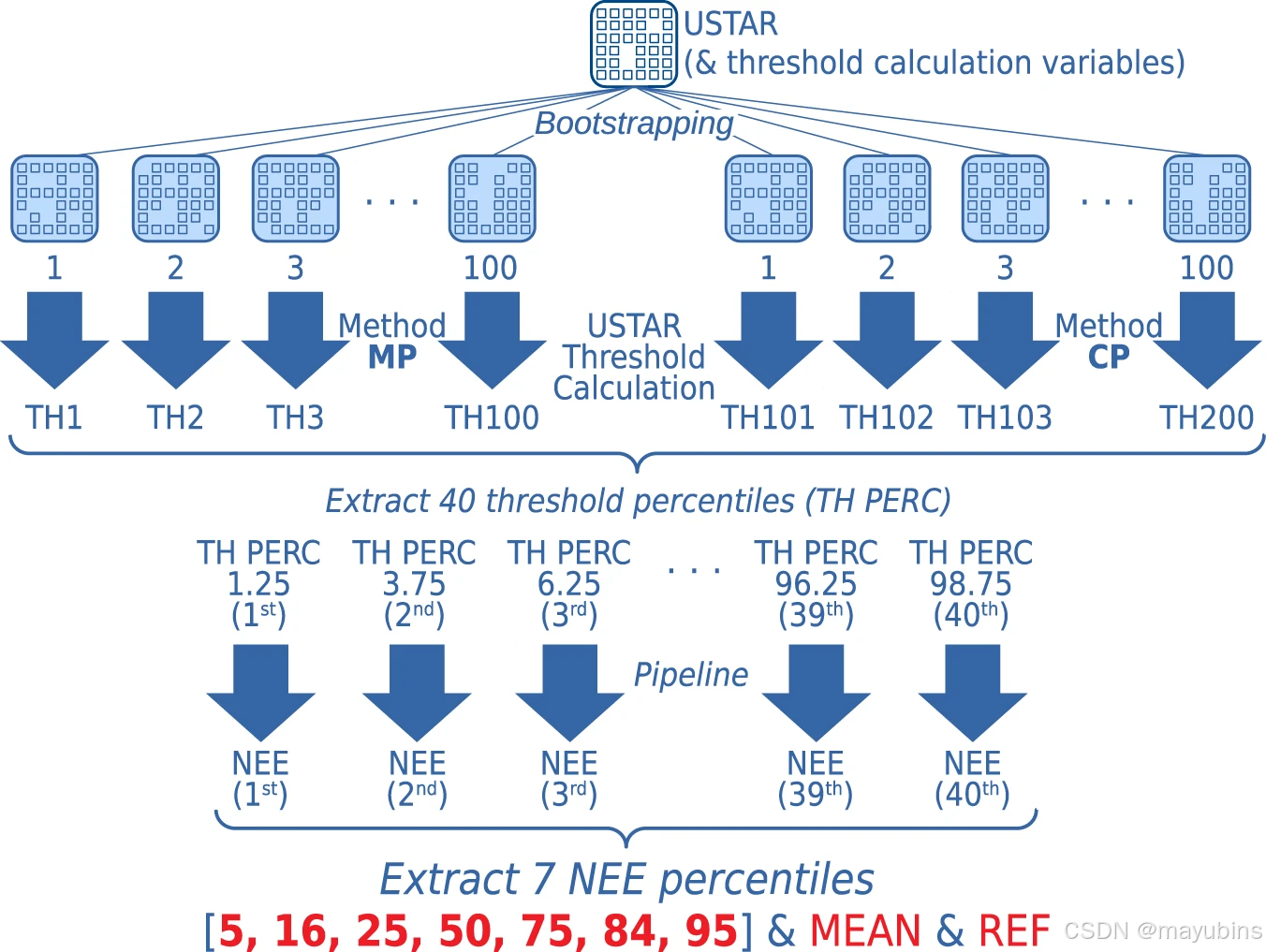
For each of the two methods, a bootstrapping technique was used. The full dataset (year of measurement) was re-sampled 100 times with the possibility to select the same data point multiple times (i.e., with replacement), creating 100 versions of the dataset. The threshold values were calculated for each of them, obtaining 100 threshold values per method (CP and MP) and year, for a total of 200 USTAR threshold estimates for each year. This process and next steps are illustrated in Fig. 3. These 200 threshold values represent the uncertainty in the threshold estimation that could also impact the uncertainty of NEE. It is worth noting that there is not always a direct relationship between the threshold and NEE uncertainties. It is possible, for instance, that a small variability in the thresholds has a strong effect on NEE or, conversely, with NEE almost insensitive to the threshold value. This is related to the site characteristics (USTAR variability) and to the level of difficulty in filling the gaps created by the filtering.对于这两种方法中的每一种，都使用了 bootstrapping 技术。完整数据集（测量年份）被重新采样 100 次，可以多次选择相同的数据点（即替换），创建 100 个版本的数据集。计算每个方法（CP 和 MP）的阈值，每个方法（CP 和 MP）和年份获得 100 个阈值，每年总共 200 个 USTAR 阈值估计值。此过程和后续步骤如图 1 所示。3. 这 200 个阈值代表了阈值估计中的不确定性，这也可能影响 NEE 的不确定性。值得注意的是，阈值和 NEE 不确定性之间并不总是有直接的关系。例如，阈值的微小变化可能对 NEE 有很强的影响，或者相反，NEE 对阈值几乎不敏感。这与场地特征（USTAR 可变性）和填补过滤产生的空白的难度有关。

To identify and remove data collected under low turbulence conditions, under which advective fluxes could lead to an underestimation of fluxes, filtering based on the USTAR threshold was used. In order to estimate the uncertainty in the USTAR threshold calculation, a bootstrapping approach was implemented, with a selection of values representative of the distribution included in the final data products. From the (up to) 200 thresholds from the combined bootstrapping of the two methods, 40 percentiles are extracted. All the subsequent steps of the pipeline are applied to all 40 versions. For each of the final output products (e.g., NEE, as illustrated here), seven percentiles representative of the distribution are included.为了识别和删除在低湍流条件下收集的数据，在低湍流条件下，平流通量可能导致低估通量，使用了基于 USTAR 阈值的过滤。为了估计 USTAR 阈值计算中的不确定性，实施了一种自举方法，其中选择代表分布的值包含在最终数据产品中。从两种方法的组合 bootstrap 的（最多）200 个阈值中，提取 40 个百分位数。管道的所有后续步骤都应用于所有 40 个版本。对于每个最终输出产品（例如 NEE，如此处所示），包括代表分布的 7 个百分位数。

There are cases where not enough data are present to calculate a USTAR threshold (for both the CP and MP methods) or where it is not possible to identify a clear change point (CP method only). This leads to the uncertainty being underestimated (fewer or no USTAR threshold values available). This should be considered as a general indication of difficulties in the application of the USTAR filtering for the specific sites or years. Sites and years where these conditions occurred are reported in the SUCCESS_RUN variable in the AUXNEE product (values 1: threshold found, 0: failed/no threshold found).在某些情况下，没有足够的数据来计算 USTAR 阈值（对于 CP 和 MP 方法），或者无法确定明确的变化点（仅限 CP 方法）。这导致不确定性被低估（可用的 USTAR 阈值较少或没有可用）。这应被视为对特定站点或年份应用 USTAR 过滤困难的一般指示。发生这些情况的地点和年份在 AUXNEE 产品的 SUCCESS_RUN 变量中报告（值 1：找到阈值，0：失败/未找到阈值）。

Variable and constant variants of the USTAR threshold methodsUSTAR 阈值方法的可变和常数变体

To calculate the uncertainty in NEE due to the uncertainty in the selected USTAR threshold, all the threshold values obtained with the two methods and the bootstrapping were pooled together, from which 40 representative values were extracted: from the percentile 1.25 of the series to the percentile 98.75, with a step of 2.5, i.e., [1.25:2.5:98.75]. When long time series (multi-years) are processed, it is possible to extract the 40 representative thresholds for each of the years. The threshold is a function of slow-changing dynamics (height of canopy, height of measurement, roughness), but a threshold changing every year could introduce false interannual variability. On the other hand, a constant threshold across all the years would not represent changes in the ecosystem structure and EC system setup. For this reason, two approaches were implemented:为了计算由于所选 USTAR 阈值的不确定性而导致的 NEE 不确定性，将使用两种方法和自举获得的所有阈值汇总在一起，从中提取了 40 个代表性值：从序列的百分位数 1.25 到百分位数 98.75，步长为 2.5，即 [1.25：2.5：98.75]。处理长时间序列（多年）时，可以提取每个年份的 40 个代表性阈值。阈值是缓慢变化的动力学（冠层高度、测量高度、粗糙度）的函数，但每年变化的阈值可能会引入错误的年际变化。另一方面，所有年份的恒定阈值并不代表生态系统结构和 EC 系统设置的变化。因此，实施了两种方法：

• Variable USTAR Threshold (VUT): The thresholds found for each year and the years immediately before and after (if available) have been pooled together, and from their joint population, the final 40 thresholds extracted. With that, the USTAR thresholds vary from year to year; however, they are still influenced by neighboring years. This is identified in FLUXNET2015 variables by the “_VUT” suffix;可变 USTAR 阈值 （VUT）：将每年以及之前和之后的年份（如果有）找到的阈值汇总在一起，并从它们的联合总体中提取出最后的 40 个阈值。因此，USTAR 阈值每年都不同;然而，它们仍然受到邻近年份的影响。这在 FLUXNET2015 变量中由 “_VUT” 后缀标识;

• Constant USTAR Threshold (CUT): Across years, all the thresholds found have been pooled together and the final 40 thresholds extracted from this dataset. With that, all years were filtered with the same USTAR threshold. This is identified in FLUXNET2015 variables by the “_CUT” suffix.恒定 USTAR 阈值 （CUT）：多年来，找到的所有阈值都被汇总在一起，并从该数据集中提取了最后 40 个阈值。这样，所有年份都使用相同的 USTAR 阈值进行筛选。这在 FLUXNET2015 变量中由 “_CUT” 后缀标识。

If the dataset includes up to two years of data, the two methods give the same result, and only the _VUT is generated.如果数据集包含最多两年的数据，则两种方法会给出相同的结果，并且只会生成_VUT。

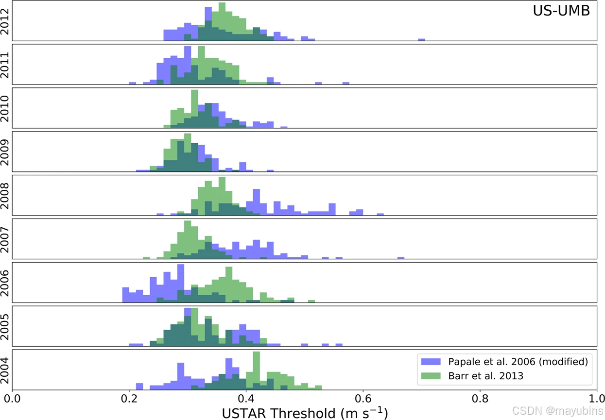
For both the VUT and CUT approaches, 40 NEE datasets have been created, filtering the original NEE time series using 40 different USTAR values estimated as explained above. The values of the thresholds are reported in the AUXNEE product file. These 40 NEE versions have been used as the basis for all the derived variables provided. An example of the variability of the two methods (CP and MP) is shown in Fig. 4, contrasting the distribution of the bootstrapped results for each method, showing comparable values for some years and divergent values for other years (of the same site). This highlights the importance of applying both methods in this ensemble-like way.对于 VUT 和 CUT 方法，已经创建了 40 个 NEE 数据集，使用如上所述估计的 40 个不同的 USTAR 值过滤原始 NEE 时间序列。阈值在 AUXNEE 产品文件中报告。这 40 个 NEE 版本已用作提供的所有派生变量的基础。两种方法（CP 和 MP）的可变性示例如图 1 所示。4，对比每种方法的 bootstrap 结果分布，显示某些年份的可比值和其他年份（同一站点）的不同值。这突出了以这种类似 ensemble 的方式应用这两种方法的重要性。

Example of the distribution of USTAR thresholds calculated for each year using the MP30 method in blue and CP41 method in green for the US-UMB site (dark green where they overlap). All these thresholds were pulled together to extract the CUT final 40 thresholds, while for the VUT thresholds, each year was pulled with the two immediately before and after (e.g., 2005 + 2006 + 2007 to extract the 40 thresholds to be used to filter 2006). Note that the level of agreement between methods and between subsequent years is variable, justifying the approach that propagates this variability into uncertainty in NEE.使用 MP30 方法（蓝色）和 CP41 方法（绿色）计算的 US-UMB 站点每年的 USTAR 阈值分布示例（重叠处为深绿色）。将所有这些阈值汇总在一起以提取 CUT 最后的 40 个阈值，而对于 VUT 阈值，每年都与紧接在前后的两个阈值一起提取（例如，2005 + 2006 + 2007 提取 40 个阈值用于过滤 2006 年）。请注意，方法之间和随后年份之间的一致性水平是可变的，这证明了将这种可变性传播到 NEE 不确定性的方法是合理的。

Filtering NEE based on USTAR thresholds根据 USTAR 阈值过滤 NEE

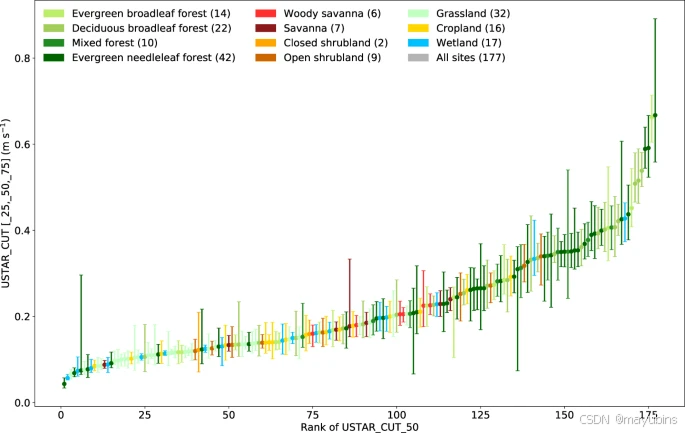
The USTAR thresholds are applied to daytime and nighttime data, removing NEE values collected when USTAR is below the threshold and removing also the first half-hour with high turbulence after a period of low turbulence to avoid false emission pulses due to CO2 accumulated under the canopy and not detected by the storage system (in particular, when a profile is not available at the site). The USTAR filtering is not applied to H and LE, because it has not been proved that when there are CO2 advective fluxes, these also impact energy fluxes, specifically due to the fact that when advection is in general large (nighttime), energy fluxes are small. Figure 5 shows the range of thresholds found (interquartile ranges) across sites in FLUXNET2015. While some sites had low thresholds and low variability in the USTAR thresholds, others show large ranges of values in some more extreme cases (indicating difficulties in estimating the “real” threshold).USTAR 阈值适用于白天和夜间数据，去除 USTAR 低于阈值时收集的 NEE 值，并去除一段时间低湍流后前半小时的高湍流，以避免由于 CO2 积聚在冠层下且未被存储系统检测到而导致错误发射脉冲（特别是， 当网站没有配置文件时）。USTAR 滤波不适用于 H 和 LE，因为尚未证明当存在 CO2 平流通量时，这些通量也会影响能量通量，特别是因为当平流通常很大（夜间）时，能量通量很小。图 5 显示了 FLUXNET2015 中各个站点找到的阈值范围（四分位距）。虽然一些站点的 USTAR 阈值阈值较低且可变性较低，但其他站点在一些更极端的情况下显示出较大的值范围（表明难以估计“实际”阈值）。

Ranked USTAR thresholds based on median threshold and error bars showing 25th to 75th percentiles of the 40 thresholds calculated with the Constant USTAR Threshold (CUT) method – only computed for sites with 3 or more years, so only 177 sites out of the 206 are shown. Colors show different ecosystem classes based on the site’s IGBP.根据中位数阈值和误差线对 USTAR 阈值进行排名，误差线显示使用恒定 USTAR 阈值 （CUT） 方法计算的 40 个阈值的th 25 个到th 75 个百分位数 - 仅针对 3 年或更长时间的站点计算，因此仅显示 206 个站点中的 177 个站点。颜色根据站点的 IGBP 显示不同的生态系统类别。

Gap-filling of NEENEE 的空白填充

Existing gaps from instrument or power failures are further increased after QC and USTAR filtering. The time series with gaps need to be filled, especially before aggregated values can be calculated (from daily to annual). Moffat et al.26 compared different gap-filling methods for CO2 concluding that most of the methods currently available perform sufficiently well with respect to the general uncertainty associated with the measurements. The method implemented here is the Marginal Distribution Sampling (MDS) method already described in the meteorological products.在 QC 和 USTAR 过滤后，仪器或电源故障造成的现有间隙会进一步增加。需要填充具有间隙的时间序列，尤其是在计算聚合值之前（从每日到每年）。Moffat 等人。26 比较了不同的 CO2 间隙填充方法，得出的结论是，目前可用的大多数方法在与测量相关的一般不确定性方面表现得足够好。这里实现的方法是气象产品中已经描述的边际分布采样 （MDS） 方法。

Selection of reference NEE variables参考 NEE 变量的选择

After filtering NEE using the 40 USTAR thresholds and gap-filling, 40 complete (gap-free) NEE time series were available for each site. For each half hour, it is possible to use the 40 values to estimate the NEE uncertainty resulting from the USTAR threshold estimation (reported as percentiles of the NEE distribution, identified by the “_XX” numeric suffix) and the average value (identified in the dataset by the “_MEAN” suffix). Since the average value has a smoothing effect on the time series, an additional reference value of NEE was selected and identified in FLUXNET2015 variables by the “_REF” suffix, in an attempt to identify which of the 40 NEE realizations was the most representative of the ensemble. The “_REF” NEE was selected among the 40 different NEE instances in this way: (1) the Nash–Sutcliffe model efficiency coefficient42 was calculated between each NEE instance and the remaining 39; (2) the reference NEE has been selected as the one with the highest model efficiency coefficients sum, i.e., the most similar to the other 39. Note that determining the reference NEE is done independently for variables using VUT and CUT USTAR thresholds, as well as for each temporal aggregation. Therefore, the version selected as REF could be different for different temporal resolutions. For instance, NEE_VUT_REF at half-hourly resolution might have been generated using a different USTAR threshold than NEE_VUT_REF at daily resolution. Information on which threshold values were used for each version and temporal aggregation can be found in the auxiliary products for NEE processing (AUXNEE). In addition to the reference NEE, the NEE instance obtained by filtering the data with the median value of the USTAR thresholds distribution is also included. This NEE is identified in FLUXNET2015 variables by the “_USTAR50” suffix (for both CP and MP methods, and both VUT and CUT approaches) and is stable across temporal aggregation resolutions. Individual percentiles of the USTAR thresholds distribution are reported in the AUXNEE file (40 instances for CUT and 40 per year for VUT).在使用 40 个 USTAR 阈值过滤 NEE 并填充间隙后，每个站点有 40 个完整（无间隙）NEE 时间序列可用。对于每半小时，可以使用 40 个值来估计由 USTAR 阈值估计（报告为 NEE 分布的百分位数，由 “_XX” 数字后缀标识）和平均值（在数据集中由 “_MEAN” 后缀标识）产生的 NEE 不确定性。由于平均值对时间序列具有平滑效应，因此在 FLUXNET2015 变量中通过“_REF”后缀选择并标识了 NEE 的附加参考值，以试图确定 40 个 NEE 实现中的哪一个最具有集成代表性。以这种方式在 40 个不同的 NEE 实例中选择“_REF”NEE：（1） 计算每个 NEE 实例与其余 39 个实例之间的 Nash-Sutcliffe 模型效率系数42;（2） 参考 NEE 被选为模型效率系数和最高的一个，即与其他 39 个最相似。请注意，对于使用 VUT 和 CUT USTAR 阈值的变量以及每个时间聚合，确定参考 NEE 是独立进行的。因此，对于不同的时间分辨率，选择为 REF 的版本可能会有所不同。例如，半小时分辨率的 NEE_VUT_REF 可能是使用与每日分辨率NEE_VUT_REF不同的 USTAR 阈值生成的。有关每个版本和时间聚合使用哪些阈值的信息，可以在 NEE 处理的辅助产品 （AUXNEE） 中找到。除了参考 NEE 之外，还包括使用 USTAR 阈值分布的中值筛选数据得到的 NEE 实例。该 NEE 在 FLUXNET2015 变量中由“_USTAR50”后缀标识（对于 CP 和 MP 方法，以及 VUT 和 CUT 方法），并且在时间聚集分辨率中保持稳定。USTAR 阈值分布的各个百分位数在 AUXNEE 文件中报告（CUT 为 40 个实例，VUT 为每年 40 个实例）。

Random uncertainty for NEENEE 的随机不确定性

In addition to the uncertainty estimates based on multiple thresholds for USTAR filtering, the random uncertainty for NEE is also estimated based on the method used by Hollinger & Richardson37. Variables expressing random uncertainty are identified by the suffix _RANDUNC. One of two methods are used to estimate random uncertainty, applied hierarchically:除了基于USTAR过滤的多个阈值的不确定性估计外，NEE的随机不确定性也根据Hollinger & Richardson37使用的方法进行估计。表示随机不确定性的变量由后缀 _RANDUNC 标识。使用以下两种方法之一来估计按层次结构应用的随机不确定性：

• NEE-RANDUNC Method 1 (direct standard deviation method): For a sliding window of ±7 days and ±1 hour of the time-of-day of the current timestamp, the random uncertainty is calculated as the standard deviation of the measured fluxes. The similarity in the meteorological conditions evaluated as in the MDS gap-filling method31 and a minimum of five measured values must be present; otherwise, method 2 is used.NEE-RANDUNC 方法 1（直接标准差法）：对于当前时间戳的 ±7 天 ±1 小时的滑动窗口，随机不确定性计算为测得磁通量的标准差。必须存在与 MDS 填隙方法31 中评估的气象条件的相似性，并且必须至少存在五个测量值;否则，使用方法 2。

• NEE-RANDUNC Method 2 (median standard deviation method): For a sliding window of ±5 days and ±1 hour of the time-of-day of the current timestamp, random uncertainty is calculated as the median of the random uncertainty (calculated with NEE-RANDUNC Method 1) of similar fluxes, i.e., within the range of ±20% and not less than 2 µmolCO2 m–2 s–1. (Note on temporal aggregations: differing sliding windows are: WW: ±2 weeks, MM: ±1 month, and YY: ±2 years.)NEE-RANDUNC 方法 2（中位数标准差法）：对于当前时间戳的 ±5 天 ±1 小时的滑动窗口，随机不确定性计算为类似通量的随机不确定性（使用 NEE-RANDUNC 方法 1 计算）的中位数，即在 ±20% 且不小于 2 μmolCO2 m–2 s–1 的范围内。（关于时间聚合的注意事项：不同的滑动窗口是：WW：±2 周，MM：±1 个月，YY：±2 年。

The joint uncertainty for NEE is computed from the combination of the uncertainty from multiple USTAR thresholds and random uncertainty. These variables identified by the _JOINTUNC suffix and are computed for NEE filtered using the VUT method as in Eq. (5), and similarly for NEE filtered with the CUT method.NEE 的联合不确定性是根据多个 USTAR 阈值的不确定性和随机不确定性的组合计算得出的。这些变量由 _JOINTUNC 后缀标识，对于使用 VUT 方法过滤的 NEE 进行计算，如方程 （5） 所示，对于使用 CUT 方法过滤的 NEE 也是如此。

NEE_VUT_REF_JOINTUNC=NEE_VUT_REF_RANDUNC2+(NEE_VUT_84−NEE_VUT_162)2

(5)

The 16th and 84th percentiles are used because they are equivalent to ±1 Standard Deviation in case of a normal distribution. (Note on temporal aggregations: joint uncertainties for NEE are recomputed at all temporal resolutions.)使用第 16 个和第 84 个百分位数，因为它们在正态分布的情况下等效于 ±1 个标准差。（关于时间聚合的注意：NEE 的联合不确定性在所有时间分辨率下都重新计算。

CO2 flux partitioning in GPP and RECOGPP 和 RECO 中的 CO2 通量分配

Partitioning CO2 fluxes from NEE into estimates of its two main components, Gross Primary Production (GPP) and Ecosystem Respiration (RECO), was done by parameterizations of models using measured data. All sites were partitioned with the nighttime fluxes method31 (_NT suffixes) and the daytime fluxes method43 (_DT suffixes), while a third method, sundown reference respiration44 (_SR suffixes), was applied to all sites meeting the method’s requirements (e.g., high quality storage measurement).通过使用测量数据对模型进行参数化，将 NEE 的 CO2 通量划分为其两个主要组成部分，即总初级生产 （GPP） 和生态系统呼吸 （RECO） 的估计值。所有站点均采用夜间通量方法31（_NT 个后缀）和白天通量方法43（_DT 个后缀）进行分区，而第三种方法，日落参考呼吸44（_SR 个后缀）应用于满足方法要求的所有站点（例如，高质量的存储测量）。

The nighttime method uses nighttime data to parameterize a respiration-temperature model that is then applied to the whole dataset to estimate RECO. GPP is then calculated as the difference between RECO and NEE. The parameterization uses short windows of time (14 days) to account for the dynamic of other important respiration drivers such as water, substrate availability, and phenology (see Reichstein et al.31 for details on the implementation and ONEFlux22 for the code).夜间方法使用夜间数据来参数化呼吸-温度模型，然后将其应用于整个数据集以估计 RECO。然后将 GPP 计算为 RECO 和 NEE 之间的差额。参数化使用较短的时间窗口（14 天）来解释其他重要呼吸驱动因素的动态，例如水、底物可用性和物候（参见 Reichstein 等人。31 了解实现的详细信息，ONEFlux22 了解代码）。

The daytime method uses daytime and nighttime data to parameterize a model with one component based on a light-response curve and vapor pressure deficit for GPP, and a second component using a respiration-temperature relationship similar to the nighttime method. In this case, NEE becomes a function of both GPP and RECO, both of which are estimated by the model. Similarly to the nighttime method, the parameterization is done for short windows (8 days) to take into consideration other slower-changing factors (see Lasslop et al.43 for details on the implementation and ONEFlux22 for the code).白天方法使用白天和夜间数据来参数化模型，其中一个分量基于 GPP 的光响应曲线和蒸气压亏缺，第二个分量使用类似于夜间方法的呼吸-温度关系。在这种情况下，NEE 成为 GPP 和 RECO 的函数，两者都由模型估计。与夜间方法类似，参数化是在短窗口（8 天）内进行的，以考虑其他变化较慢的因素（参见 Lasslop 等人。43 了解实现的详细信息，ONEFlux22 了解代码）。

For forest sites where a CO2 concentration profile for storage fluxes was available, an additional RECO estimate was calculated using the method from van Gorsel et al.44, with variables identified by the _SR suffix. In this method, the parameterization of a respiration-temperature model is based solely on data acquired just after sundown, aiming at excluding the measurements potentially affected by advection and also assuming that in the first hour of the evening the advective transport is not yet established.对于有 CO2 储存通量浓度曲线的林地，使用 van Gorsel 等人的方法计算了额外的 RECO 估计值。44，变量由 _SR 后缀标识。在这种方法中，呼吸温度模型的参数化完全基于日落后获取的数据，旨在排除可能受平流影响的测量值，并假设在傍晚的第一个小时内平流传输尚未建立。

The sundown partitioning method requires that the NEE is not filtered for low turbulence conditions (USTAR), and for this reason it was applied only to the original time series. The nighttime and daytime methods instead require NEE filtered for low turbulence conditions. For this reason they were applied to all the 40 NEE versions resulting from the 40 USTAR thresholds, obtaining 40 versions of GPP and RECO for each of the two partitioning methods, propagating the uncertainty from NEE to GPP and RECO. This has been done for both the CUT and VUT filtering methods.日落分区方法要求不对低湍流条件 （USTAR） 的 NEE 进行过滤，因此它仅应用于原始时间序列。相反，夜间和白天方法需要针对低湍流条件进行 NEE 滤波。因此，它们被应用于由 40 个 USTAR 阈值产生的所有 40 个 NEE 版本，为两种分区方法中的每一种获得 40 个 GPP 和 RECO 版本，将不确定性从 NEE 传播到 GPP 和 RECO。CUT 和 VUT 滤波方法都已完成此作。

Similarly to NEE, the 40 GPP and RECO estimates (for each method and for CUT and VUT) have been used to calculate the percentiles of their distribution for each timestep (describing their uncertainty due to the NEE uncertainty). The average value (_MEAN) and the reference value use the same model efficiency approach used for NEE for each temporal aggregation. Similarly, NEE filtered with the median USTAR value (_USTAR50) has been partitioned into GPP and RECO. Information on the threshold values used for all versions of GPP and RECO (_NT and _DT, _VUT and _CUT, HH to YY resolutions) are in the auxiliary files for NEE processing (AUXNEE). Variables for reference GPP and RECO are also identified by a _REF suffix. The two methods for the partitioning (three for the cases in which the sundown method is applied) are not merged in any way, because their difference is informative with the respect to the uncertainty of the methods, as in the case of a model comparison exercise.与 NEE 类似，40 GPP 和 RECO 估计值（对于每种方法以及 CUT 和 VUT）已用于计算它们在每个时间步长的分布百分位数（描述由于 NEE 不确定性而导致的不确定性）。平均值 （_MEAN） 和参考值对每个时间聚合使用用于 NEE 的相同模型效率方法。同样，使用中位 USTAR 值 （_USTAR50） 过滤的 NEE 已划分为 GPP 和 RECO。有关用于所有版本的 GPP 和 RECO（_NT 和 _DT、_VUT 和 _CUT、HH 到 YY 分辨率）的阈值的信息，请参见 NEE 处理 （AUXNEE） 的辅助文件。参考 GPP 和 RECO 的变量也由 _REF 后缀标识。两种分割方法（在应用 sundown 方法的情况下为 3 种）不会以任何方式合并，因为它们的差异对于方法的不确定性提供了信息，就像在模型比较练习的情况下一样。

Implementation approach实施方法

To increase the traceability of changes between versions of datasets and reduce uncertainty stemming from choices made at implementation time, we favored using original code implementations or thoroughly validated re-implementations of original codes. Thus, our code organization strings together loosely coupled components which implement each step, with clear-cut interfaces between steps. This modular approach eases the maintenance and change efforts for any individual step, but adds complexity to evaluating changes for the entire pipeline. Different programming languages (Python, C, MATLAB and IDL, plus PV-WAVE for FLUXNET2015) were used to implement the different steps, all connected using a controller code that makes appropriate calls in the correct order. The ONEFlux22 code collection replaced the PV-WAVE code with a re-implementation in Python, and also collates most of these steps into a cohesive pipeline (see also the Code Availability section). The IDL code, which applies the sundown partitioning method44, is not yet currently implemented in ONEFlux, because some additional testing and development are needed to make it robust and more suitable for general application. Implementation details of individual steps are discussed next, with references to the outputs each step identified by an execution sequential number and the step name–e.g., 01_qc_visual contains the results of the first processing step, the visual check step. Each of these steps correspond to a code module. Supplementary Fig. SM2 shows the steps and their inter-dependencies.为了提高数据集版本之间更改的可追溯性并减少在实施时所做的选择所带来的不确定性，我们倾向于使用原始代码实现或经过全面验证的原始代码的重新实现。因此，我们的代码组织将实现每个步骤的松散耦合组件串在一起，步骤之间具有明确的接口。这种模块化方法简化了任何单个步骤的维护和变更工作，但增加了评估整个管道变更的复杂性。使用不同的编程语言（Python、C、MATLAB 和 IDL，以及 FLUXNET2015的 PV-WAVE）来实现不同的步骤，所有步骤都使用控制器代码进行连接，该代码以正确的顺序进行适当的调用。ONEFlux22 代码集合用 Python 重新实现取代了 PV-WAVE 代码，并将这些步骤中的大部分整理到一个内聚的管道中（另请参阅代码可用性部分）。应用 sundown 分区方法44 的 IDL 代码目前尚未在 ONEFlux 中实现，因为需要一些额外的测试和开发来使其健壮且更适合一般应用。接下来将讨论各个步骤的实施细节，并引用输出，每个步骤由执行序列号和步骤名称标识，例如，01_qc_visual包含第一个处理步骤（可视化检查步骤）的结果。这些步骤中的每一个都对应于一个代码模块。补充图SM2 显示了步骤及其相互依赖关系。

Steps implemented in python在 python 中实现的步骤

The main controller code for ONEFlux is implemented in Python. Besides being the glue code that executes each step, pre- and post-checks are also executed before and after each step. These checks guarantee that the input data meet the minimum requirements to run the step, that the minimum expected outputs were generated by the execution of the step, and that any errors or exception conditions were handled correctly. Information about execution is recorded in a log for the entire pipeline, along with logs for individual steps. Besides the controller code, two of the three flux partitioning steps were re-implemented in Python (the nighttime and daytime methods, 10_nee_partition_nt and 11_nee_partition_dt), together with other specific steps such as data preparation for the uncertainty estimates (12_ure_input), and the creation and checking of final products (99_fluxnet2015). The original flux partitioning implementation in PV-WAVE was used for the LaThuile2007 and FLUXNET2015 datasets. Also, the tool for the downscaling of the ERA-I meteorological data is implemented in Python and runs on a server connected to the ERA data.ONEFlux 的主控制器代码是用 Python 实现的。除了作为执行每个步骤的胶水代码外，每个步骤之前和之后还会执行前检查和后检查。这些检查可保证输入数据满足运行步骤的最低要求，执行步骤时生成了最低预期输出，并且正确处理了任何错误或异常情况。有关执行的信息记录在整个管道的日志中，以及各个步骤的日志中。除了控制器代码之外，三个通量分区步骤中的两个在 Python 中重新实现（夜间和白天方法、10_nee_partition_nt 和 11_nee_partition_dt），以及其他特定步骤，例如不确定性估计 （12_ure_input） 的数据准备以及最终产品的创建和检查（99_fluxnet2015）。PV-WAVE 中最初的通量分区实现用于 LaThuile2007 和 FLUXNET2015 数据集。此外，用于缩小 ERA-I 气象数据比例的工具是在 Python 中实现的，并在连接到 ERA 数据的服务器上运行。

Steps implemented in C在 C 语言中实现的步骤

Several steps are implemented in the C programming language, allowing better control over execution performance of these steps. These steps include:使用 C 编程语言实现了几个步骤，从而可以更好地控制这些步骤的执行性能。这些步骤包括：

automated QA/QC flagging (02_qc_auto), USTAR threshold estimation using the MP method (04_ustar_mp), the filtering and gap-filling of meteorological data, including the merging with the ERA-I downscaled data (07_meteo_proc), the filtering and gap-filling of CO2 fluxes (08_nee_proc), the filtering, gap-filling, and energy corrections of energy fluxes (09_energy_proc), and the computation of uncertainty products (12_ure). The source codes and the compiled executables are provided for steps implemented in C, as well as build procedures in make/Makefile format.自动 QA/QC 标记 （02_qc_auto），使用 MP 方法进行 USTAR 阈值估计 （04_ustar_mp），气象数据的过滤和间隙填充，包括与 ERA-I 缩小数据的合并 （07_meteo_proc），CO2 通量的过滤和间隙填充 （08_nee_proc），能量通量的过滤、间隙填充和能量校正 （09_energy_proc）， 以及不确定性产品的计算 （12_ure）。源代码和编译的可执行文件是为用 C 语言实现的步骤以及 make/Makefile 格式的构建过程提供的。

Steps implemented in MATLAB在 MATLAB 中实现的步骤

The estimation of USTAR thresholds using the CP method (05_ustar_cp) is the only step implemented in MATLAB. It is distributed both as source code and compiled code to be used with the MATLAB Runtime Environment, such that it does not require a license purchase.使用 CP 方法 （05_ustar_cp） 估计 USTAR 阈值是在 MATLAB 中实现的唯一步骤。它以源代码和编译代码的形式分发，以便与 MATLAB 运行时环境一起使用，因此不需要购买许可证。

Data Records数据记录

The FLUXNET2015 portion presented in this paper contains 1496 site-years of data from 206 sites45,46,47,48,49,50,51,52,53,54,55,56,57,58,59,60,61,62,63,64,65,66,67,68,69,70,71,72,73,74,75,76,77,78,79,80,81,82,83,84,85,86,87,88,89,90,91,92,93,94,95,96,97,98,99,100,101,102,103,104,105,106,107,108,109,110,111,112,113,114,115,116,117,118,119,120,121,122,123,124,125,126,127,128,129,130,131,132,133,134,135,136,137,138,139,140,141,142,143,144,145,146,147,148,149,150,151,152,153,154,155,156,157,158,159,160,161,162,163,164,165,166,167,168,169,170,171,172,173,174,175,176,177,178,179,180,181,182,183,184,185,186,187,188,189,190,191,192,193,194,195,196,197,198,199,200,201,202,203,204,205,206,207,208,209,210,211,212,213,214,215,216,217,218,219,220,221,222,223,224,225,226,227,228,229,230,231,232,233,234,235,236,237,238,239,240,241,242,243,244,245,246,247,248,249,250, characterizing ecosystem-level carbon and energy fluxes in diverse ecosystems across the globe (Fig. 1, Supplementary Fig. SM1251,252), spanning from the early 1990s to 2014, with 69 sites having decade-long records. The dataset covers the distribution of ecosystem fluxes as reported in the recent meta-analyses253,254 (Fig. 6).本文介绍的FLUXNET2015部分包含来自 206 个站点的 1496 个站点年的数据45、46、47、48、49、50、51、52、53、54、55、56、57、58、59、60、61、62、63、64、65、66、67、68、69,70,71,72,73,74,75,76,77,78,79,80,81,82,83,84,85,86,87,88,89,90,91,92,93,94,95,96，97,98,99,100,101,102,103,104,105,106,107,108,109,110,111,112,113,114,115,116,117,118,119,120,121,122,123，124,125,126,127,128,129,130,131,132,133,134,135,136,137,138,139,140,141,142,143,144,145,146,147,148，票价：149,150,151,152,153,154,155,156,157,158,159,160,161,162,163,164,165,166,167,168,169,170,171,172，173,174,175,176,177,178,179,180,181,182,183,184,185,186,187,188,189,190,191,192,193,194,195,196，197,198,199,200,201,202,203,204,205,206,207,208,209,210,211,212,213,214,215,216,217,218,219，220,221,222,223,224,225,226,227,228,229,230,231,232,233,234,235,236,237,238,239,240,241,242,243，244,245,246,247,248,249,250，表征了全球不同生态系统中生态系统层面的碳和能量通量（图 .1、补充图SM1251,252），从 1990 年代初到 2014 年，有 69 个站点拥有长达十年的记录。该数据集涵盖了最近的荟萃分析253,254 中报告的生态系统通量分布（图 D）。6）.

Fig. 6图 6

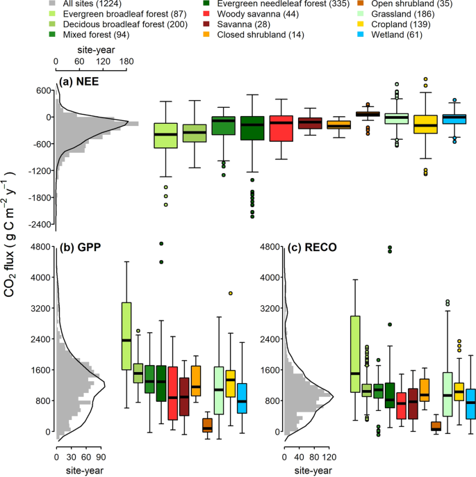
Distribution of the yearly (a) net ecosystem exchange (NEE), (b) gross primary production (GPP), and (c) ecosystem respiration (RECO) in FLUXNET2015. Only data with QC flag (NEE_VUT_REF_QC) higher than 0.5 are shown here. The values are reference NEE, GPP, and RECO based on the Variable USTAR Threshold (VUT) and selected reference for model efficiency (REF). GPP and RECO are based on the nighttime partitioning (NT) method. The grey histogram (bin width 100 gC m−2 y−1) shows the flux distribution in 1224 of the available site-years; negative GPP and RECO values are kept to preserve distributions, see Data processing methods section for details. Black lines show the distribution curves based on published data253,254. The boxplots show the flux distribution (i.e., 25th, 50th, and 75th percentiles) for vegetation types defined and color-coded according to IGBP (International Geosphere–Biosphere Programme) definitions. Circles represent data points beyond the 1.5-times interquartile range (25th to 75th percentile) plus the 75th percentile or minus 25th percentile (whisker). Numbers in parentheses indicate the number of site-years used in each IGBP group. The NO-Blv site from the snow/ice IGBP group is not shown in the boxplots.FLUXNET2015 年年度 （a） 生态系统净交换 （NEE）、（b） 总初级生产力 （GPP） 和 （c） 生态系统呼吸 （RECO） 的分布。此处仅显示 QC 标志 （NEE_VUT_REF_QC） 高于 0.5 的数据。这些值是基于可变 USTAR 阈值 （VUT） 的参考 NEE、GPP 和 RECO 以及模型效率的选定参考 （REF）。GPP 和 RECO 基于夜间分区 （NT） 方法。灰色直方图（区间宽度 100 gC m−2 y−1）显示了 1224 个可用站点年份的通量分布;保留负 GPP 和 RECO 值以保留分布，有关详细信息，请参阅数据处理方法部分。黑线表示基于已发布数据253,254 的分布曲线。箱线图显示了根据 IGBP（国际地圈-生物圈计划）定义和颜色编码的植被类型的通量分布（即第 25、50 和 75 个百分位数）。圆圈表示超出 1.5 倍四分位距（第 25 个百分位到第 75 个百分位）加上第 75 个百分位或负第 25 个百分位（须线）的数据点。括号中的数字表示每个 IGBP 组中使用的站点年数。来自雪/冰 IGBP 组的 NO-Blv 站点未显示在箱线图中。

Full size image全尺寸图像

The dataset is distributed in files separated by sites, by temporal aggregation resolutions (e.g., hourly, weekly), and by data products (e.g., FULLSET with all the variables and SUBSET designed for less experienced users). All data files for a site are available for download as a single ZIP file archive with site-specific DOI. The file-naming conventions details these options for each file (Table 1). Site metadata are also available as a single file containing metadata for all sites, detailed later in this section and Supplementary Table SM8. Note that DOIs are assigned at the site level, one DOI per site for all of that site’s products. A DOI was not assigned to the whole FLUXNET2015 dataset, since this would make citation and assigning credit imprecise and hard to track.数据集分布在按站点、时间聚合分辨率（例如，每小时、每周）和数据产品（例如，具有所有变量的 FULLSET 和专为经验不足的用户设计的 SUBSET）分隔的文件中。站点的所有数据文件都可以作为单个 ZIP 文件存档下载，其中包含特定于站点的 DOI。文件命名约定详细说明了每个文件的这些选项（表 1）。站点元数据也作为包含所有站点元数据的单个文件提供，本节稍后将详细介绍和补充表 SM8。请注意，DOI 是在站点级别分配的，每个站点对应该站点的所有商品 1 个 DOI。没有为整个 FLUXNET2015 数据集分配 DOI，因为这会使引用和分配信用不精确且难以跟踪。

Table 1 The template of file naming conventions, including the field, field definition, and the possible options.表 1 文件命名约定的模板，包括字段、字段定义和可能的选项。

Full size table全尺寸表格

The FLUXNET2015 dataset provides data at five temporal resolutions. Site teams contribute either half-hourly (HH) or hourly (HR) datasets, depending on the integration/aggregation time decided by the site managers and function of the characteristics of the turbulence. References to half-hourly in this paper also apply to hourly data, unless explicitly stated otherwise. Half-hourly data are the basis of all the processing done for this dataset and are the finest grained temporal resolution provided. Coarser aggregations are generated uniformly from half-hourly data within the data processing pipeline. The other standard temporal aggregations are: daily (DD), weekly (WW), monthly (MM), and yearly (YY).FLUXNET2015 数据集提供 5 种时间分辨率的数据。现场团队贡献半小时 （HH） 或每小时 （HR） 数据集，具体取决于现场经理决定的集成/聚合时间和湍流特征的功能。除非另有明确说明，否则本文中对半小时数据的引用也适用于每小时数据。半小时数据是为此数据集完成的所有处理的基础，并且是提供的最精细的时间分辨率。较粗的聚合是从数据处理管道中的半小时数据统一生成的。其他标准时间聚合为：每日 （DD）、每周 （WW）、每月 （MM） 和每年 （YY）。

The complete output from the data processing pipeline includes over 200 variables–among which are measured and derived data, quality flags, uncertainty quantification variables, and results from intermediate data processing steps. The variable names follow the naming conventions of <BASENAME>_<QUALIFIER>, where BASENAME describes the physical quantities (e.g., TA, NEE, Table 2) and QUALIFIER describes the information of processing methods (e.g., VUT, CUT), uncertainties (e.g., RANDUNC), and quality flags (e.g., QC) (see Supplementary Table SM1).数据处理管道的完整输出包括 200 多个变量，其中包括测量和派生数据、质量标志、不确定性量化变量以及中间数据处理步骤的结果。变量名称遵循 _ 的命名约定<BASENAME><QUALIFIER>，其中 BASENAME 描述物理量（例如，TA、NEE、表 2），QUALIFIER 描述处理方法（例如，VUT、CUT）、不确定性（例如，RANDUNC）和质量标志（例如，QC）的信息（参见补充表 SM1）。

Table 2 List of the variable basenames, descriptions, available resolutions and units.表 2 变量基本名称、描述、可用分辨率和单位的列表。

Full size table全尺寸表格

To serve the users with an easier-to-use data product, we created two variants with different selections of variables for data distribution: the FULLSET with all the results and variables; and the SUBSET, designed to help non-expert users, with a reduced set of variables that should fit most needs.为了为用户提供更易于使用的数据产品，我们创建了两个变体，其中包含用于数据分配的不同变量选择：包含所有结果和变量的 FULLSET;以及 SUBSET，旨在帮助非专家用户，其减少的变量集应该可以满足大多数需求。

• FULLSET: variables generated by the processing such as uncertainty quantification variables, all variants of the data products, all quality information flags, and many variables generated by intermediate processing steps to allow in-depth understanding of individual processing steps and their effect in the final data products. A summary of the main variable basenames is in Table 2, while a full list of variables is provided in Supplementary Table SM1. Key features of the FULLSET version are:FULLSET：由处理生成的变量，例如不确定性量化变量、数据产品的所有变体、所有质量信息标志以及中间处理步骤生成的许多变量，以便深入了解各个处理步骤及其在最终数据产品中的影响。表 2 中总结了主要变量碱基名称，而补充表 SM1 中提供了完整的变量列表。FULLSET 版本的主要特点是：

  • Meteorological variables filled with multiple gap-filling methods (e.g., MDS, ERA) are provided separately.用多种间隙填充方法（例如 MDS、ERA）填充的气象变量单独提供。

  • NEE versions filtered with two different methods of extracting the USTAR thresholds (i.e., CUT, VUT) are provided. Multiple percentiles and reference NEE are also provided.提供了使用两种不同方法提取 USTAR 阈值（即 CUT、VUT）过滤的 NEE 版本。还提供了多个百分位数和参考 NEE。

  • GPP and RECO partitioned from NEE filtered with VUT and CUT methods, using both daytime and nighttime partitioning methods (i.e., NT, DT). Multiple percentiles and reference GPP and RECO are provided.使用白天和夜间分区方法（即 NT、DT）从 NEE 中通过 VUT 和 CUT 方法过滤的 GPP 和 RECO 进行分区。提供了多个百分位数和参考 GPP 和 RECO。

  • LE and H gap-filled, adjusted and non-adjusted for energy balance closure, are both provided.同时提供 LE 和 H 间隙填充、调整和非调整能量平衡闭合。

  • Random, methodological, and joint uncertainties for NEE, GPP, RECO, LE, and H are provided.提供了 NEE、GPP、RECO、LE 和 H 的随机、方法和联合不确定性。

• SUBSET: Includes a subset of the data product. The selection of the variables for this data product was done based on the expected usage for most users and to help less experienced users. Although the number of variables used is reduced, they are still accompanied by a set of quality flags and uncertainty quantification variables essential to correctly interpret the data. Key features of the SUBSET version are:SUBSET：包括数据产品的子集。此数据产品的变量选择是根据大多数用户的预期使用情况完成的，旨在帮助经验不足的用户。尽管使用的变量数量减少了，但它们仍然伴随着一组质量标志和不确定性量化变量，这对于正确解释数据至关重要。SUBSET 版本的主要功能包括：

  • Only the consolidated gap-filled meteorological variables are provided.仅提供合并的间隙填充气象变量。

  • Only the REF version of NEE filtered with the VUT method is provided. Selected percentiles and reference NEE are also provided.仅提供使用 VUT 方法过滤的 NEE 的 REF 版本。此外，还提供了选定的百分位数和参考 NEE。

  • GPP and RECO (only REF versions) partitioned from NEE filtered with only the VUT method, using both daytime and nighttime partitioning methods, are provided. Selected percentiles and reference GPP and RECO are also provided.提供了 GPP 和 RECO （仅限 REF 版本），仅使用 VUT 方法从 NEE 过滤，同时使用白天和夜间分区方法。此外，还提供了选定的百分位数以及参考 GPP 和 RECO。

  • LE and H gap-filled, adjusted and non-adjusted for energy balance closure, are both provided.同时提供 LE 和 H 间隙填充、调整和非调整能量平衡闭合。

  • Random and methodological uncertainties for NEE, GPP, RECO, LE, and H are provided.提供了 NEE、GPP、RECO、LE 和 H 的随机和方法不确定性。

The variable proposed in the SUBSET product is NEE_VUT_REF since it maintains the temporal variability (as opposed to the MEAN NEE), it is representative of the ensemble, and the VUT method is sensitive to possible changes of the canopy (density and height) and site setup, which can have an impact on the turbulence and consequently on the USTAR threshold. The RECO and GPP products in SUBSET are calculated from the corresponding NEE variables filtered with the VUT method, generating RECO_NT_VUT_REF and RECO_DT_VUT_REF for RECO, and GPP_NT_VUT_REF and GPP_DT_VUT_REF for GPP. It is important to use both daytime (DT) and nighttime (NT) variables, and consider their difference as uncertainty.SUBSET 产品中提出的变量是 NEE_VUT_REF，因为它保持时间变化（与 MEAN NEE 相反），它代表集成，并且 VUT 方法对冠层（密度和高度）和站点设置的可能变化很敏感，这可能会对湍流产生影响，从而影响 USTAR 阈值。SUBSET 中的 RECO 和 GPP 产品是根据使用 VUT 方法过滤的相应 NEE 变量计算得出的，为 RECO 生成RECO_NT_VUT_REF和RECO_DT_VUT_REF，为 GPP 生成 GPP_NT_VUT_REF 和 GPP_DT_VUT_REF。请务必同时使用白天 （DT） 和夜间 （NT） 变量，并将它们的差异视为不确定性。

Auxiliary data products provide extra information on specific parameters of the data processing pipeline. The groups of products are:辅助数据产品提供有关数据处理管道特定参数的额外信息。产品组包括：

• AUXMETEO: Auxiliary data product containing information about the downscaling of meteorological variables using the ERA-Interim reanalysis data product (TA, PA, VPD, WS, P, SW_IN, and LW_IN). Variables in these files relate to the linear regression and error/correlation estimates for each data variable used in the downscaling.AUXMETEO：辅助数据产品，包含有关使用 ERA-Interim 再分析数据产品（TA、PA、VPD、WS、P、SW_IN 和 LW_IN）缩小气象变量的信息。这些文件中的变量与缩减中使用的每个数据变量的线性回归和误差/相关性估计值相关。

  • Parameters:参数：

    • ERA_SLOPE: the slope of linear regressionERA_SLOPE：线性回归的斜率

    • ERA_INTERCEPT: intercept point of linear regressionERA_INTERCEPT：线性回归的截距点

    • ERA_RMSE: root mean square error between site data and downscaled data

    • ERA_CORRELATION: correlation coefficient of linear fitERA_CORRELATION：线性拟合的相关系数

• AUXNEE: Auxiliary data product with variables resulting from the processing of NEE (mainly related to USTAR filtering) and generation of RECO and GPP. Variables in this product include success/failure of execution of USTAR filtering methods, USTAR thresholds applied to different versions of variables, and percentile/threshold pairs with best model efficiency results.AUXNEE：辅助数据产品，其变量由 NEE 处理（主要与 USTAR 滤波有关）和 RECO 和 GPP 的生成产生。本产品中的变量包括 USTAR 筛选方法执行成功/失败、应用于不同版本变量的 USTAR 阈值以及具有最佳模型效率结果的百分位数/阈值对。

  • Variables:变量：

    • USTAR_MP_METHOD: Moving Point Test USTAR threshold method runUSTAR_MP_METHOD：移动点测试 USTAR 阈值方法运行

    • USTAR_CP_METHOD: Change Point Detection USTAR threshold method runUSTAR_CP_METHOD：变化点检测 USTAR 阈值方法运行

    • NEE_USTAR50_[UT]: 50th percentile of USTAR thresholds obtained from bootstrapping and sed to generate NEE_USTAR50_[UT] (with UT either CUT or VUT)NEE_USTAR50_[UT]：从 bootstrap 和 sed 获取的 USTAR 阈值的第 50 个百分位数，以生成 NEE_USTAR50_[UT]（UT 为 CUT 或 VUT）

    • NEE_[UT]_REF: USTAR threshold used to calculate the reference NEE, using model efficiency approach (with UT either CUT or VUT)NEE_[UT]_REF：用于计算参考 NEE 的 USTAR 阈值，使用模型效率方法（UT 为 CUT 或 VUT）

    • [PROD]_[ALG]_[UT]_REF: USTAR threshold used to filter the NEE that was used to produce the reference product PROD (RECO or GPP), selected using model efficiency approach, using algorithm ALG (NT, DT) (with UT either CUT or VUT)[PROD]_[ALG]_[UT]_REF：用于过滤用于生成参考产品 PROD（RECO 或 GPP）的 NEE 的 USTAR 阈值，使用模型效率方法选择，使用算法 ALG（NT、DT）（UT 为 CUT 或 VUT）

  • Parameters:参数：

    • SUCCESS_RUN: 1 if a run of a method (USTAR_MP_METHOD or USTAR_CP_METHOD) was successful, 0 otherwiseSUCCESS_RUN：如果方法（USTAR_MP_METHOD 或 USTAR_CP_METHOD）运行成功，则为 1，否则为 0

    • USTAR_PERCENTILE: percentile of USTAR thresholds from bootstrapping at USTAR filtering stepUSTAR_PERCENTILE：USTAR 筛选步骤中自举的 USTAR 阈值百分位数

    • USTAR_THRESHOLD: USTAR threshold value corresponding to USTAR_PERCENTILEUSTAR_THRESHOLD：对应于 USTAR_PERCENTILE 的 USTAR 阈值

    • [RR]_USTAR_PERCENTILE: percentile of USTAR thresholds from bootstrapping at USTAR filtering step at resolution RR (HH, DD, WW, MM, YY)[RR]_USTAR_PERCENTILE：分辨率 RR 时 USTAR 滤波步长自举的 USTAR 阈值百分位数（HH、DD、WW、MM、YY）

    • [RR]_USTAR_THRESHOLD: USTAR threshold value corresponding to USTAR_PERCENTILE at resolution RR (HH, DD, WW, MM, YY)[RR]_USTAR_THRESHOLD：分辨率 RR 时对应于USTAR_PERCENTILE的 USTAR 阈值（HH、DD、WW、MM、YY）

• ERAI: Auxiliary data product containing full record (1989–2014) of downscaled meteorological variables using the ERA-Interim reanalysis data product, including TA, PA, VPD, WS, P, SW_IN, and LW_IN.ERAI：辅助数据产品，包含使用 ERA-Interim 再分析数据产品缩小的气象变量的全记录 （1989-2014），包括 TA、PA、VPD、WS、P、SW_IN 和 LW_IN。

The FLUXNET2015 metadata are included in a single file (FLX_AA-Flx_BIF_[RESOLUTION]_[YYYYMMDD].xlsx) for all sites for each data product resolution (see Table 1 for resolution options). The metadata follow the Biological, Ancillary, Disturbance, and Metadata (BADM255,256) standards and are provided in the BADM Interchange Format29 (BIF). Table 3 illustrates the type of metadata included with selected metadata variables (See full lists and descriptions of the metadata in Supplementary Tables SM2–SM7). Height and instrument models for the flux variables, as well as soil temperature and moisture depths, are reported in the Variable Information metadata.对于每个数据产品分辨率，FLUXNET2015元数据都包含在一个文件 （FLX_AA-Flx_BIF_[RESOLUTION]_[YYYYMMDD].xlsx） 中（有关分辨率选项，请参阅表 1）。元数据遵循生物、辅助、干扰和元数据 （BADM255,256） 标准，并以 BADM 交换格式29 （BIF） 提供。表 3 说明了所选元数据变量中包含的元数据类型（请参阅补充表 SM2–SM7 中元数据的完整列表和说明）。通量变量的高度和仪器模型以及土壤温度和湿度深度都在变量信息元数据中报告。

Table 3 Metadata types and selected variables. See Supplementary Tables SM2–SM7 for a full list of metadata with descriptions. Variables collected from or generated for all sites are in bold.表 3 元数据类型和所选变量。有关元数据的完整列表和说明，请参阅补充表 SM2–SM7。从所有站点收集或为所有站点生成的变量以粗体显示。

Full size table全尺寸表格

Technical Validation技术验证

Eddy covariance measurements offer a direct method to estimate trace gas or energy exchanges between surface and atmosphere at an ecosystem scale (approximately up to 1 km around the measurement point). This makes eddy covariance difficult to compare with other methods. Nonetheless, eddy covariance data have been extensively used in numerous scientific papers and studies that indirectly validate their reliability and usefulness. Hundreds of articles have been published based on eddy covariance measurements; examples of multi-site studies using FLUXNET2015 data include Jung et al.15, Tramontana et al.257, and Keenan et al.258.涡度相关测量提供了一种在生态系统尺度（测量点周围约 1 公里）估计地表和大气之间的痕量气体或能量交换的直接方法。这使得涡度协方差很难与其他方法进行比较。尽管如此，涡度相关数据已被广泛用于许多科学论文和研究，间接验证了它们的可靠性和有用性。已经发表了数百篇基于涡度相关测量的文章;使用 FLUXNET2015 数据的多中心研究示例包括 Jung 等人。15， Tramontana 等人。257 和 Keenan 等人。258.

Eddy covariance data were evaluated with respect to other methods such as inventory and chambers by Campioli et al.259, who showed that “EC [eddy covariance] biases are not apparent across sites, suggesting the effectiveness of standard post-processing procedures. Our results increase confidence in EC …”. The approach of Campioli et al.259 requires sites that have several additional (and rare) pieces of information; therefore, it is not generally applicable, particularly not across the sites used in this study. However, the eddy covariance site teams co-authoring this paper have compared and technically validated their measurements with respect to knowledge of their site. Unavoidably, measurement and processing uncertainties exist, and can be large for certain sites and ecosystem conditions. However, in general, flux values provided in this dataset are consistent with expectations, and eddy covariance remains one of the more reliable techniques for assessing land-air exchanges at ecosystem scales.Campioli 等人根据其他方法（如库存和腔室）评估了涡度协方差数据。259 人指出，“EC [涡度相关] 偏差在各个站点之间并不明显，这表明标准后处理程序的有效性。我们的结果增加了对 EC 的信心......”。Campioli 等人的方法。259 要求网站包含几条额外的（和罕见的）信息;因此，它通常不适用，尤其是在本研究中使用的站点中。然而，本文的合著者涡度相关站点团队已经比较并技术验证了他们关于站点知识的测量值。不可避免地，存在测量和处理的不确定性，并且对于某些地点和生态系统条件来说可能很大。然而，总的来说，该数据集中提供的通量值与预期一致，涡度协方差仍然是评估生态系统尺度上陆地-空气交换的更可靠的技术之一。

Usage Notes使用说明

Detailed documentation on how to use and interpret FLUXNET2015 is available online at FLUXNET2015 Dataset - FLUXNET. Here, we present some of the main points to guide the usage of the data.有关如何使用和解释 FLUXNET2015 的详细文档，请访问 FLUXNET2015 Dataset - FLUXNET。在这里，我们提出了一些要点来指导数据的使用。

Risks in the application of standard procedures应用标准程序的风险

When standardized procedures are applied across different sites, the possible differences owing to data treatment are avoided or minimized; this is one of the main goals of FLUXNET2015 and ONEFlux. However, there is also the risk and possibility that the standard methods don’t work properly or as expected at specific sites and under certain conditions. This is particularly true for the CO2 flux partitioning, which as with all models is based on assumptions that could not always be not valid. For this reason, it could be necessary to contact the site PIs that are listed in Supplementary Table SM9.当标准化程序应用于不同地点时，可以避免或最大限度地减少由于数据处理而可能产生的差异;这是 FLUXNET2015 和 ONEFlux 的主要目标之一。但是，也存在标准方法在特定地点和特定条件下无法正常工作或无法按预期工作的风险和可能性。对于 CO2 通量分配尤其如此，与所有模型一样，它基于并不总是无效的假设。因此，可能需要联系补充表 SM9 中列出的研究中心 PI。

Using the QC flags使用 QC 标志

There are quality-control flag variables in the dataset to help users filter and interpret variables, especially for gap-filled and process knowledge-based variables. These flags are described in the variable documentation (Supplementary Table SM1). It is highly recommended that one carefully considers the QC flags when using the data.数据集中有质量控制标志变量，可帮助用户筛选和解释变量，尤其是对于间隙填充和流程基于知识的变量。这些标志在变量文档（补充表 SM1）中进行了描述。强烈建议在使用数据时仔细考虑 QC 标志。

Percentile variants for fluxes and reference values磁通量和参考值的百分位数变体

For most flux variables, there are reference values and percentile versions of the variables to help understand some of the uncertainty in the record. For NEE, RECO, and GPP, the percentiles are generated from the bootstrapping of the USTAR threshold estimation step, i.e., they characterize the variability from a range of values obtained as USTAR thresholds. In addition, three different reference values are provided (“_MEAN”, “_USTAR50” and “_REF”) in order to cover different user needs. In general the “_REF” version should be the most representative, particularly if related to the percentiles. It is, however, important to clearly refer to which NEE version is used in order to ensure reproducibility. For the energy balance corrected H and LE variables, the percentiles indicate the variability due to the uncertainty in the correction factor applied. Similarly to NEE, there are gap-filled and energy balance corrected versions of H and LE variables; therefore, it is also important to clearly refer to which version is used. The SUBSET version of the dataset includes a reduced number of variables, selected for non-expert users. We encourage users to carefully evaluate their requirements and options in the dataset, and if needed to contact regional networks, site teams, or even co-authors of this article for help and recommendations. For more detail, see the Methods section above.对于大多数通量变量，都有变量的参考值和百分位数版本，以帮助理解记录中的一些不确定性。对于 NEE、RECO 和 GPP，百分位数是由 USTAR 阈值估计步骤的自举生成的，即，它们从作为 USTAR 阈值获得的一系列值中表征可变性。此外，提供三种不同的参考值（“_MEAN”、“_USTAR50”和“_REF”），以涵盖不同的用户需求。一般来说，“_REF”版本应该是最具代表性的，特别是当与百分位数相关时。然而，重要的是要清楚地说明使用的 NEE 版本，以确保可重复性。对于能量平衡校正的 H 和 LE 变量，百分位数表示由于应用的校正因子的不确定性而导致的变异性。与 NEE 类似，H 和 LE 变量有间隙填充和能量平衡校正版本;因此，明确引用使用的版本也很重要。数据集的 SUBSET 版本包含为非专家用户选择的变量数量减少。我们鼓励用户仔细评估他们在数据集中的要求和选项，如果需要，请联系区域网络、站点团队，甚至是本文的合著者寻求帮助和建议。有关更多详细信息，请参阅上面的 Methods 部分。

Temporally aggregated resolutions时间聚合的决议

All data products are provided at multiple temporal resolutions where feasible. The finest resolution is either hourly or half-hourly (indicated by the filename tags HR and HH, respectively). These data are then aggregated into daily (DD), 7-day weekly (WW), monthly (MM), and yearly (YY) resolutions, with appropriate aggregations for each variable, such as averaging for TA and summation for P.在可行的情况下，所有数据产品都以多种时间分辨率提供。最佳分辨率为每小时或半小时（分别由文件名标记 HR 和 HH 表示）。然后将这些数据聚合为每日 （DD）、7 天每周 （WW）、每月 （MM） 和每年 （YY） 分辨率，并为每个变量进行适当的聚合，例如 TA 的平均值和 P 的求和。

Timestamps时间 戳

Timestamps in the data and metadata files use the format YYYYMMDDHHMM, truncated at the appropriate resolution (e.g., YYYYMMDD for a date or YYYYMM for a month). Two formats of time associated with a record are used: (1) single timestamp, where the meaning of the timestamp is unambiguous, and, (2) a pair of timestamps, indicating the start and end of the period the timestamps represent.数据和元数据文件中的时间戳使用 YYYYMMDDHHMM 格式，并以适当的分辨率截断（例如，YYYYMMDD 表示日期，YYYYMM 表示一个月）。使用与记录关联的两种时间格式：（1） 单个时间戳，其中时间戳的含义明确，以及 （2） 一对时间戳，指示时间戳所表示的时间段的开始和结束。

Time zones时区

To allow more direct site comparability, all time variables are reported in local standard time (i.e., without daylight saving time). The time zone information with respect to UTC time is reported in the site metadata.为了实现更直接的站点可比性，所有时间变量都以当地标准时间报告（即没有夏令时）。与 UTC 时间相关的时区信息在站点元数据中报告。

Numeric resolution数字分辨率

The floating point numbers are maintained at their original resolution throughout processing steps, using double precision for the majority of cases, and are truncated at up to nine decimal places in the distributed files for numbers between 0.0 and 1.0, and at up to five decimal places for larger numbers.浮点数在整个处理步骤中保持其原始分辨率，在大多数情况下使用双精度，对于介于 0.0 和 1.0 之间的数字，在分布式文件中最多截断 9 位小数，对于较大的数字，最多截断 5 位小数。

Column ordering列排序

The order of columns is not always the same in different files (e.g., different sites). User data-processing routines should use the variable label (which is always consistent) and not the order of occurrence of that variable in the file. Timestamps are the only exception and will always be the first variable(s)/column(s) of the data file. This applies to text file data representations (i.e., CSV formatted).在不同的文件（例如，不同的站点）中，列的顺序并不总是相同的。用户数据处理例程应使用变量标签（始终一致），而不是该变量在文件中的出现顺序。时间戳是唯一的例外，并且始终是数据文件的第一个变量/列。这适用于文本文件数据表示形式（即 CSV 格式）。

Missing data缺失数据

Missing data values are indicated with −9999, without decimal points, independent of the cause of the missing value.缺失数据值以 −9999 表示，不含小数点，与缺失值的原因无关。

Known issues已知问题

A list of known issues and limitations relevant to the dataset is maintained online: Known Issues - FLUXNET.与数据集相关的已知问题和限制列表在线维护：Known Issues - FLUXNET。

Releases of the FLUXNET2015 datasetFLUXNET2015 数据集的发布

The original FLUXNET2015 release was in December 2015, followed by incremental releases in July 2016 and November 2016, and, finally, a release in February 2020 with fixes and additional metadata as described in this paper. More information on the releases can be found in the online change log: Data Change Log - FLUXNET. A newer release replaces all previous ones, and only the newest release is available for direct download. Access to previous versions can be obtained upon request.最初的FLUXNET2015版本于 2015 年 12 月发布，随后在 2016 年 7 月和 2016 年 11 月发布增量版本，最后在 2020 年 2 月发布，其中包含本文中所述的修复和其他元数据。有关版本的更多信息，请参阅在线更改日志：Data Change Log - FLUXNET。较新的版本将替换所有以前的版本，并且只有最新版本可以直接下载。可应要求访问以前的版本。

Support to FLUXNET2015 data users对 FLUXNET2015 数据用户的支持

Scientists and staff responsible for the creation of the dataset offer support to data users and can be reached at fluxdata-support@fluxdata.org.负责创建数据集的科学家和工作人员为数据用户提供支持，可通过 fluxdata-support@fluxdata.org 联系。

Updates and future versions更新和未来版本

There is strong interest and engagement in order to ensure the availability of new data (new sites and new years), keeping the open policy and the high quality data that we tried to reach with this work. We expect that the processing pipeline and QA/QC procedures will continue evolving, in support of new products. However, the amount of both technical and coordination work, along with difficulty securing long-term international funding, hamper creation of new versions of the dataset. There are ongoing discussions among regional networks and FLUXNET on this coordination, but currently there is no plan for a follow-up version of FLUXNET2015.为了确保新数据（新站点和新年份）的可用性，保持开放的政策和我们试图通过这项工作获得的高质量数据，人们表现出了强烈的兴趣和参与。我们预计加工流程和 QA/QC 程序将继续发展，以支持新产品。然而，技术和协调工作量以及难以获得长期国际资金，阻碍了数据集新版本的创建。区域网络和 FLUXNET 之间正在就此协调进行讨论，但目前没有 FLUXNET2015 后续版本的计划。

Code availability代码可用性

The ONEFlux collection of codes used to create data intercomparable with FLUXNET2015 has been packaged to be executed as a complete pipeline and is available in both source-code and executable forms under a 3-clause BSD license on GitHub: https://github.com/AmeriFlux/ONEFlux. The complete environment to run this pipeline requires a GCC compatible C compiler (or capability to run pre-compiled Windows, Linux, and/or Mac executables), a MATLAB Runtime Environment, and a Python interpreter with a few numeric and scientific packages installed. All of these can be obtained at no cost.用于创建与 FLUXNET2015 互连的数据的 ONEFlux 代码集合已被打包为作为完整的管道执行，并且在 GitHub 上根据 3 条款 BSD 许可证以源代码和可执行形式提供：https://github.com/AmeriFlux/ONEFlux。运行此管道的完整环境需要一个兼容 GCC 的 C 编译器（或运行预编译的 Windows、Linux 和/或 Mac 可执行文件的功能）、一个 MATLAB 运行时环境以及一个安装了一些数值和科学软件包的 Python 解释器。所有这些都可以免费获得。

Change history更改历史记录

• 25 February 2021

  A Correction to this paper has been published: Author Correction: The FLUXNET2015 dataset and the ONEFlux processing pipeline for eddy covariance data | Scientific Data

  25 二月 2021

  本文的更正已发布：Author Correction: The FLUXNET2015 dataset and the ONEFlux processing pipeline for eddy covariance data | Scientific Data

• 26 February 2021

  A Correction to this paper has been published: Author Correction: The FLUXNET2015 dataset and the ONEFlux processing pipeline for eddy covariance data | Scientific Data

  26 二月 2021

  本文的更正已发布：Author Correction: The FLUXNET2015 dataset and the ONEFlux processing pipeline for eddy covariance data | Scientific Data

DEEPSEEK对文章的总结和使用数据建议

文献总结

这篇文献介绍了FLUXNET2015数据集及其处理流程ONEFlux。FLUXNET2015是一个全球性的生态系统尺度数据集，涵盖了212个站点的CO₂、水和能量交换数据，以及其他气象和生物测量数据。数据集的时间跨度从1990年代到2014年，包含了超过1500个站点年的数据。该数据集通过统一的处理方法和质量控制流程，确保了数据的一致性和可比性。FLUXNET2015数据集首次包含了超过20年的长期记录，并且206个站点的数据首次以**Creative Commons (CC-BY 4.0)**许可证发布。

数据集的主要应用包括生态生理学研究、遥感研究以及生态系统和地球系统模型的开发。FLUXNET2015还提供了衍生数据产品，如填补缺失数据的时间序列、生态系统呼吸和光合作用估算、不确定性估计等。

关键建议

1. 理解数据集的组成和结构：

   • FLUXNET2015数据集包含了多个时间分辨率的数据（半小时、小时、日、周、月、年），并且每个站点都有多个变量（如CO₂通量、能量通量、气象变量等）。

   • 数据集分为FULLSET和SUBSET两个版本。FULLSET包含所有变量和处理步骤的详细信息，适合高级用户；SUBSET则是一个简化版本，适合非专业用户。

2. 关注数据质量标志（QC Flags）：

   • 数据集中每个变量都有相关的质量标志（QC Flags），用于指示数据的质量（如是否填补、填补的置信度等）。在使用数据时，务必检查这些标志，以确保数据的可靠性。

   • 例如，NEE_VUT_REF_QC标志用于指示净生态系统交换（NEE）的质量，值越高表示数据质量越好。

3. 注意不确定性估计：

   • FLUXNET2015提供了多种不确定性估计方法，特别是对于CO₂通量的不确定性（如USTAR阈值的不确定性）。在使用数据时，建议考虑这些不确定性，尤其是在进行模型验证或生态系统碳平衡研究时。

   • 例如，NEE_VUT_REF_JOINTUNC变量提供了NEE的联合不确定性估计，结合了随机不确定性和方法不确定性。

4. 选择合适的通量分区方法：

   • FLUXNET2015提供了多种CO₂通量分区方法（如夜间法、白天法、日落参考呼吸法）。不同的方法可能适用于不同的生态系统类型和研究目的。建议根据研究需求选择合适的通量分区方法。

   • 例如，GPP_NT_VUT_REF和GPP_DT_VUT_REF分别表示基于夜间法和白天法的总初级生产力（GPP）估算。

5. 使用辅助数据产品：

   • FLUXNET2015还提供了辅助数据产品（如AUXNEE和AUXMETEO），这些产品包含了处理过程中的中间结果和元数据。这些数据可以帮助用户更好地理解数据处理流程和结果的来源。

   • 例如，AUXNEE文件包含了USTAR阈值的信息，可以帮助用户理解CO₂通量过滤的不确定性。

6. 注意时间戳和时区：

   • 数据集中的所有时间戳都使用本地标准时间（无夏令时）。在使用数据时，务必注意时间戳的时区信息，以确保时间序列的正确性。

   • 例如，UTC_OFFSET变量提供了站点相对于UTC的时区偏移量。

7. 处理缺失数据：

   • 数据集中的缺失数据用-9999表示。在进行数据分析时，需要处理这些缺失值，以避免对结果产生偏差。

8. 参考FLUXNET2015的在线文档：

   • FLUXNET2015提供了详细的在线文档和使用指南，建议在使用数据前仔细阅读这些文档，以了解数据集的具体内容和处理方法。

   • 文档链接：FLUXNET2015 Dataset Documentation

总结

FLUXNET2015是一个强大的全球生态系统数据集，适用于多种生态学和气候研究。在使用该数据集时，建议用户仔细阅读文档，理解数据的处理流程和质量控制方法，特别是关注数据质量标志和不确定性估计。通过合理选择通量分区方法和辅助数据产品，可以更好地利用该数据集进行科学研究。