


Deep Reinforcement Learning: Pong from Pixels
This is a long overdue blog post on Reinforcement Learning (RL). RL is hot! You may have noticed that computers can now automatically learn to play ATARI games (from raw game pixels!), they are beating world champions at Go, simulated quadrupeds are learning to run and leap, and robots are learning how to perform complex manipulation tasks that defy explicit programming. It turns out that all of these advances fall under the umbrella of RL research. I also became interested in RL myself over the last ~year: I worked through Richard Sutton’s book, read through David Silver’s course, watched John Schulmann’s lectures, wrote an RL library in Javascript, over the summer interned at DeepMind working in the DeepRL group, and most recently pitched in a little with the design/development of OpenAI Gym, a new RL benchmarking toolkit. So I’ve certainly been on this funwagon for at least a year but until now I haven’t gotten around to writing up a short post on why RL is a big deal, what it’s about, how it all developed and where it might be going.

It’s interesting to reflect on the nature of recent progress in RL. I broadly like to think about four separate factors that hold back AI:
- Compute (the obvious one: Moore’s Law, GPUs, ASICs),
- Data (in a nice form, not just out there somewhere on the internet - e.g. ImageNet),
- Algorithms (research and ideas, e.g. backprop, CNN, LSTM), and
- Infrastructure (software under you - Linux, TCP/IP, Git, ROS, PR2, AWS, AMT, TensorFlow, etc.).
Similar to what happened in Computer Vision, the progress in RL is not driven as much as you might reasonably assume by new amazing ideas. In Computer Vision, the 2012 AlexNet was mostly a scaled up (deeper and wider) version of 1990’s ConvNets. Similarly, the ATARI Deep Q Learning paper from 2013 is an implementation of a standard algorithm (Q Learning with function approximation, which you can find in the standard RL book of Sutton 1998), where the function approximator happened to be a ConvNet. AlphaGo uses policy gradients with Monte Carlo Tree Search (MCTS) - these are also standard components. Of course, it takes a lot of skill and patience to get it to work, and multiple clever tweaks on top of old algorithms have been developed, but to a first-order approximation the main driver of recent progress is not the algorithms but (similar to Computer Vision) compute/data/infrastructure.
Now back to RL. Whenever there is a disconnect between how magical something seems and how simple it is under the hood I get all antsy and really want to write a blog post. In this case I’ve seen many people who can’t believe that we can automatically learn to play most ATARI games at human level, with one algorithm, from pixels, and from scratch - and it is amazing, and I’ve been there myself! But at the core the approach we use is also really quite profoundly dumb (though I understand it’s easy to make such claims in retrospect). Anyway, I’d like to walk you through Policy Gradients (PG), our favorite default choice for attacking RL problems at the moment. If you’re from outside of RL you might be curious why I’m not presenting DQN instead, which is an alternative and better-known RL algorithm, widely popularized by the ATARI game playing paper. It turns out that Q-Learning is not a great algorithm (you could say that DQN is so 2013 (okay I’m 50% joking)). In fact most people prefer to use Policy Gradients, including the authors of the original DQN paper who have shown Policy Gradients to work better than Q Learning when tuned well. PG is preferred because it is end-to-end: there’s an explicit policy and a principled approach that directly optimizes the expected reward. Anyway, as a running example we’ll learn to play an ATARI game (Pong!) with PG, from scratch, from pixels, with a deep neural network, and the whole thing is 130 lines of Python only using numpy as a dependency (Gist link). Lets get to it.
Pong from pixels


The game of Pong is an excellent example of a simple RL task. In the ATARI 2600 version we’ll use you play as one of the paddles (the other is controlled by a decent AI) and you have to bounce the ball past the other player (I don’t really have to explain Pong, right?). On the low level the game works as follows: we receive an image frame (a 210x160x3 byte array (integers from 0 to 255 giving pixel values)) and we get to decide if we want to move the paddle UP or DOWN (i.e. a binary choice). After every single choice the game simulator executes the action and gives us a reward: Either a +1 reward if the ball went past the opponent, a -1 reward if we missed the ball, or 0 otherwise. And of course, our goal is to move the paddle so that we get lots of reward.
As we go through the solution keep in mind that we’ll try to make very few assumptions about Pong because we secretly don’t really care about Pong; We care about complex, high-dimensional problems like robot manipulation, assembly and navigation. Pong is just a fun toy test case, something we play with while we figure out how to write very general AI systems that can one day do arbitrary useful tasks.
Policy network. First, we’re going to define a policy network that implements our player (or “agent”). This network will take the state of the game and decide what we should do (move UP or DOWN). As our favorite simple block of compute we’ll use a 2-layer neural network that takes the raw image pixels (100,800 numbers total (210*160*3)), and produces a single number indicating the probability of going UP. Note that it is standard to use a stochastic policy, meaning that we only produce a probability of moving UP. Every iteration we will sample from this distribution (i.e. toss a biased coin) to get the actual move. The reason for this will become more clear once we talk about training.

and to make things concrete here is how you might implement this policy network in Python/numpy. Suppose we’re given a vector x that holds the (preprocessed) pixel information. We would compute:
h = np.dot(W1, x) # compute hidden layer neuron activations
h[h<0] = 0 # ReLU nonlinearity: threshold at zero
logp = np.dot(W2, h) # compute log probability of going up
p = 1.0 / (1.0 + np.exp(-logp)) # sigmoid function (gives probability of going up)
where in this snippet W1 and W2 are two matrices that we initialize randomly. We’re not using biases because meh. Notice that we use the sigmoid non-linearity at the end, which squashes the output probability to the range [0,1]. Intuitively, the neurons in the hidden layer (which have their weights arranged along the rows of W1) can detect various game scenarios (e.g. the ball is in the top, and our paddle is in the middle), and the weights in W2can then decide if in each case we should be going UP or DOWN. Now, the initial random W1 and W2 will of course cause the player to spasm on spot. So the only problem now is to find W1 and W2 that lead to expert play of Pong!
Fine print: preprocessing. Ideally you’d want to feed at least 2 frames to the policy network so that it can detect motion. To make things a bit simpler (I did these experiments on my Macbook) I’ll do a tiny bit of preprocessing, e.g. we’ll actually feed difference frames to the network (i.e. subtraction of current and last frame).
It sounds kind of impossible. At this point I’d like you to appreciate just how difficult the RL problem is. We get 100,800 numbers (210*160*3) and forward our policy network (which easily involves on order of a million parameters in W1 and W2). Suppose that we decide to go UP. The game might respond that we get 0 reward this time step and gives us another 100,800 numbers for the next frame. We could repeat this process for hundred timesteps before we get any non-zero reward! E.g. suppose we finally get a +1. That’s great, but how can we tell what made that happen? Was it something we did just now? Or maybe 76 frames ago? Or maybe it had something to do with frame 10 and then frame 90? And how do we figure out which of the million knobs to change and how, in order to do better in the future? We call this the credit assignment problem. In the specific case of Pong we know that we get a +1 if the ball makes it past the opponent. The true cause is that we happened to bounce the ball on a good trajectory, but in fact we did so many frames ago - e.g. maybe about 20 in case of Pong, and every single action we did afterwards had zero effect on whether or not we end up getting the reward. In other words we’re faced with a very difficult problem and things are looking quite bleak.
Supervised Learning. Before we dive into the Policy Gradients solution I’d like to remind you briefly about supervised learning because, as we’ll see, RL is very similar. Refer to the diagram below. In ordinary supervised learning we would feed an image to the network and get some probabilities, e.g. for two classes UP and DOWN. I’m showing log probabilities (-1.2, -0.36) for UP and DOWN instead of the raw probabilities (30% and 70% in this case) because we always optimize the log probability of the correct label (this makes math nicer, and is equivalent to optimizing the raw probability because log is monotonic). Now, in supervised learning we would have access to a label. For example, we might be told that the correct thing to do right now is to go UP (label 0). In an implementation we would enter gradient of 1.0 on the log probability of UP and run backprop to compute the gradient vector [Math Processing Error]∇Wlogp(y=UP∣x). This gradient would tell us how we should change every one of our million parameters to make the network slightly more likely to predict UP. For example, one of the million parameters in the network might have a gradient of -2.1, which means that if we were to increase that parameter by a small positive amount (e.g. 0.001), the log probability of UP would decrease by 2.1 * 0.001 (decrease due to the negative sign). If we then did a parameter update then, yay, our network would now be slightly more likely to predict UP when it sees a very similar image in the future.
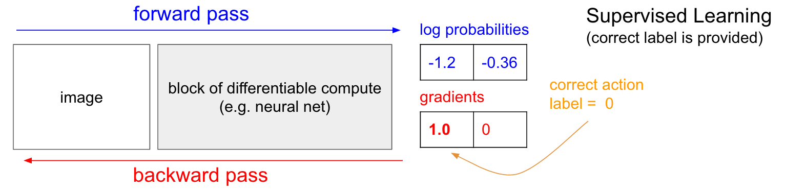
Policy Gradients. Okay, but what do we do if we do not have the correct label in the Reinforcement Learning setting? Here is the Policy Gradients solution (again refer to diagram below). Our policy network calculated probability of going UP as 30% (logprob -1.2) and DOWN as 70% (logprob -0.36). We will now sample an action from this distribution; E.g. suppose we sample DOWN, and we will execute it in the game. At this point notice one interesting fact: We could immediately fill in a gradient of 1.0 for DOWN as we did in supervised learning, and find the gradient vector that would encourage the network to be slightly more likely to do the DOWN action in the future. So we can immediately evaluate this gradient and that’s great, but the problem is that at least for now we do not yet know if going DOWN is good. But the critical point is that that’s okay, because we can simply wait a bit and see! For example in Pong we could wait until the end of the game, then take the reward we get (either +1 if we won or -1 if we lost), and enter that scalar as the gradient for the action we have taken (DOWN in this case). In the example below, going DOWN ended up to us losing the game (-1 reward). So if we fill in -1 for log probability of DOWN and do backprop we will find a gradient that discourages the network to take the DOWN action for that input in the future (and rightly so, since taking that action led to us losing the game).

And that’s it: we have a stochastic policy that samples actions and then actions that happen to eventually lead to good outcomes get encouraged in the future, and actions taken that lead to bad outcomes get discouraged. Also, the reward does not even need to be +1 or -1 if we win the game eventually. It can be an arbitrary measure of some kind of eventual quality. For example if things turn out really well it could be 10.0, which we would then enter as the gradient instead of -1 to start off backprop. That’s the beauty of neural nets; Using them can feel like cheating: You’re allowed to have 1 million parameters embedded in 1 teraflop of compute and you can make it do arbitrary things with SGD. It shouldn’t work, but amusingly we live in a universe where it does.
Training protocol. So here is how the training will work in detail. We will initialize the policy network with some W1, W2 and play 100 games of Pong (we call these policy “rollouts”). Lets assume that each game is made up of 200 frames so in total we’ve made 20,000 decisions for going UP or DOWN and for each one of these we know the parameter gradient, which tells us how we should change the parameters if we wanted to encourage that decision in that state in the future. All that remains now is to label every decision we’ve made as good or bad. For example suppose we won 12 games and lost 88. We’ll take all 200*12 = 2400 decisions we made in the winning games and do a positive update (filling in a +1.0 in the gradient for the sampled action, doing backprop, and parameter update encouraging the actions we picked in all those states). And we’ll take the other 200*88 = 17600 decisions we made in the losing games and do a negative update (discouraging whatever we did). And… that’s it. The network will now become slightly more likely to repeat actions that worked, and slightly less likely to repeat actions that didn’t work. Now we play another 100 games with our new, slightly improved policy and rinse and repeat.
Policy Gradients: Run a policy for a while. See what actions led to high rewards. Increase their probability.

If you think through this process you’ll start to find a few funny properties. For example what if we made a good action in frame 50 (bouncing the ball back correctly), but then missed the ball in frame 150? If every single action is now labeled as bad (because we lost), wouldn’t that discourage the correct bounce on frame 50? You’re right - it would. However, when you consider the process over thousands/millions of games, then doing the first bounce correctly makes you slightly more likely to win down the road, so on average you’ll see more positive than negative updates for the correct bounce and your policy will end up doing the right thing.
Update: December 9, 2016 - alternative view. In my explanation above I use the terms such as “fill in the gradient and backprop”, which I realize is a special kind of thinking if you’re used to writing your own backprop code, or using Torch where the gradients are explicit and open for tinkering. However, if you’re used to Theano or TensorFlow you might be a little perplexed because the code is oranized around specifying a loss function and the backprop is fully automatic and hard to tinker with. In this case, the following alternative view might be more intuitive. In vanilla supervised learning the objective is to maximize [Math Processing Error]∑ilogp(yi∣xi) where [Math Processing Error]xi,yi are training examples (such as images and their labels). Policy gradients is exactly the same as supervised learning with two minor differences: 1) We don’t have the correct labels [Math Processing Error]yi so as a “fake label” we substitute the action we happened to sample from the policy when it saw [Math Processing Error]xi, and 2) We modulate the loss for each example multiplicatively based on the eventual outcome, since we want to increase the log probability for actions that worked and decrease it for those that didn’t. So in summary our loss now looks like [Math Processing Error]∑iAilogp(yi∣xi), where [Math Processing Error]yi is the action we happened to sample and [Math Processing Error]Ai is a number that we call an advantage. In the case of Pong, for example, [Math Processing Error]Ai could be 1.0 if we eventually won in the episode that contained [Math Processing Error]xiand -1.0 if we lost. This will ensure that we maximize the log probability of actions that led to good outcome and minimize the log probability of those that didn’t. So reinforcement learning is exactly like supervised learning, but on a continuously changing dataset (the episodes), scaled by the advantage, and we only want to do one (or very few) updates based on each sampled dataset.
More general advantage functions. I also promised a bit more discussion of the returns. So far we have judged the goodness of every individual action based on whether or not we win the game. In a more general RL setting we would receive some reward [Math Processing Error]rt at every time step. One common choice is to use a discounted reward, so the “eventual reward” in the diagram above would become [Math Processing Error]Rt=∑k=0∞γkrt+k, where [Math Processing Error]γ is a number between 0 and 1 called a discount factor (e.g. 0.99). The expression states that the strength with which we encourage a sampled action is the weighted sum of all rewards afterwards, but later rewards are exponentially less important. In practice it can can also be important to normalize these. For example, suppose we compute [Math Processing Error]Rt for all of the 20,000 actions in the batch of 100 Pong game rollouts above. One good idea is to “standardize” these returns (e.g. subtract mean, divide by standard deviation) before we plug them into backprop. This way we’re always encouraging and discouraging roughly half of the performed actions. Mathematically you can also interpret these tricks as a way of controlling the variance of the policy gradient estimator. A more in-depth exploration can be found here.
Deriving Policy Gradients. I’d like to also give a sketch of where Policy Gradients come from mathematically. Policy Gradients are a special case of a more general score function gradient estimator. The general case is that when we have an expression of the form [Math Processing Error]Ex∼p(x∣θ)[f(x)] - i.e. the expectation of some scalar valued score function [Math Processing Error]f(x) under some probability distribution [Math Processing Error]p(x;θ) parameterized by some [Math Processing Error]θ. Hint hint, [Math Processing Error]f(x) will become our reward function (or advantage function more generally) and [Math Processing Error]p(x) will be our policy network, which is really a model for [Math Processing Error]p(a∣I), giving a distribution over actions for any image [Math Processing Error]I. Then we are interested in finding how we should shift the distribution (through its parameters [Math Processing Error]θ) to increase the scores of its samples, as judged by [Math Processing Error]f (i.e. how do we change the network’s parameters so that action samples get higher rewards). We have that:
[Math Processing Error]∇θEx[f(x)]=∇θ∑xp(x)f(x)definition of expectation=∑x∇θp(x)f(x)swap sum and gradient=∑xp(x)∇θp(x)p(x)f(x)both multiply and divide by p(x)=∑xp(x)∇θlogp(x)f(x)use the fact that ∇θlog(z)=1z∇θz=Ex[f(x)∇θlogp(x)]definition of expectationTo put this in English, we have some distribution [Math Processing Error]p(x;θ) (I used shorthand [Math Processing Error]p(x) to reduce clutter) that we can sample from (e.g. this could be a gaussian). For each sample we can also evaluate the score function [Math Processing Error]f which takes the sample and gives us some scalar-valued score. This equation is telling us how we should shift the distribution (through its parameters [Math Processing Error]θ) if we wanted its samples to achieve higher scores, as judged by [Math Processing Error]f. In particular, it says that look: draw some samples [Math Processing Error]x, evaluate their scores [Math Processing Error]f(x), and for each [Math Processing Error]x also evaluate the second term [Math Processing Error]∇θlogp(x;θ). What is this second term? It’s a vector - the gradient that’s giving us the direction in the parameter space that would lead to increase of the probability assigned to an [Math Processing Error]x. In other words if we were to nudge [Math Processing Error]θ in the direction of [Math Processing Error]∇θlogp(x;θ) we would see the new probability assigned to some [Math Processing Error]x slightly increase. If you look back at the formula, it’s telling us that we should take this direction and multiply onto it the scalar-valued score [Math Processing Error]f(x). This will make it so that samples that have a higher score will “tug” on the probability density stronger than the samples that have lower score, so if we were to do an update based on several samples from [Math Processing Error]p the probability density would shift around in the direction of higher scores, making highly-scoring samples more likely.

I hope the connection to RL is clear. Our policy network gives us samples of actions, and some of them work better than others (as judged by the advantage function). This little piece of math is telling us that the way to change the policy’s parameters is to do some rollouts, take the gradient of the sampled actions, multiply it by the score and add everything, which is what we’ve done above. For a more thorough derivation and discussion I recommend John Schulman’s lecture.
Learning. Alright, we’ve developed the intuition for policy gradients and saw a sketch of their derivation. I implemented the whole approach in a 130-line Python script, which uses OpenAI Gym’s ATARI 2600 Pong. I trained a 2-layer policy network with 200 hidden layer units using RMSProp on batches of 10 episodes (each episode is a few dozen games, because the games go up to score of 21 for either player). I did not tune the hyperparameters too much and ran the experiment on my (slow) Macbook, but after training for 3 nights I ended up with a policy that is slightly better than the AI player. The total number of episodes was approximately 8,000 so the algorithm played roughly 200,000 Pong games (quite a lot isn’t it!) and made a total of ~800 updates. I’m told by friends that if you train on GPU with ConvNets for a few days you can beat the AI player more often, and if you also optimize hyperparameters carefully you can also consistently dominate the AI player (i.e. win every single game). However, I didn’t spend too much time computing or tweaking, so instead we end up with a Pong AI that illustrates the main ideas and works quite well:
The learned agent (in green, right) facing off with the hard-coded AI opponent (left).
Learned weights. We can also take a look at the learned weights. Due to preprocessing every one of our inputs is an 80x80 difference image (current frame minus last frame). We can now take every row of W1, stretch them out to 80x80 and visualize. Below is a collection of 40 (out of 200) neurons in a grid. White pixels are positive weights and black pixels are negative weights. Notice that several neurons are tuned to particular traces of bouncing ball, encoded with alternating black and white along the line. The ball can only be at a single spot, so these neurons are multitasking and will “fire” for multiple locations of the ball along that line. The alternating black and white is interesting because as the ball travels along the trace, the neuron’s activity will fluctuate as a sine wave and due to the ReLU it would “fire” at discrete, separated positions along the trace. There’s a bit of noise in the images, which I assume would have been mitigated if I used L2 regularization.

What isn’t happening
So there you have it - we learned to play Pong from from raw pixels with Policy Gradients and it works quite well. The approach is a fancy form of guess-and-check, where the “guess” refers to sampling rollouts from our current policy, and the “check” refers to encouraging actions that lead to good outcomes. Modulo some details, this represents the state of the art in how we currently approach reinforcement learning problems. Its impressive that we can learn these behaviors, but if you understood the algorithm intuitively and you know how it works you should be at least a bit disappointed. In particular, how does it not work?
Compare that to how a human might learn to play Pong. You show them the game and say something along the lines of “You’re in control of a paddle and you can move it up and down, and your task is to bounce the ball past the other player controlled by AI”, and you’re set and ready to go. Notice some of the differences:
- In practical settings we usually communicate the task in some manner (e.g. English above), but in a standard RL problem you assume an arbitrary reward function that you have to discover through environment interactions. It can be argued that if a human went into game of Pong but without knowing anything about the reward function (indeed, especially if the reward function was some static but random function), the human would have a lot of difficulty learning what to do but Policy Gradients would be indifferent, and likely work much better. Similarly, if we took the frames and permuted the pixels randomly then humans would likely fail, but our Policy Gradient solution could not even tell the difference (if it’s using a fully connected network as done here).
- A human brings in a huge amount of prior knowledge, such as intuitive physics (the ball bounces, it’s unlikely to teleport, it’s unlikely to suddenly stop, it maintains a constant velocity, etc.), and intuitive psychology (the AI opponent “wants” to win, is likely following an obvious strategy of moving towards the ball, etc.). You also understand the concept of being “in control” of a paddle, and that it responds to your UP/DOWN key commands. In contrast, our algorithms start from scratch which is simultaneously impressive (because it works) and depressing (because we lack concrete ideas for how not to).
- Policy Gradients are a brute force solution, where the correct actions are eventually discovered and internalized into a policy. Humans build a rich, abstract model and plan within it. In Pong, I can reason that the opponent is quite slow so it might be a good strategy to bounce the ball with high vertical velocity, which would cause the opponent to not catch it in time. However, it also feels as though we also eventually “internalize” good solutions into what feels more like a reactive muscle memory policy. For example if you’re learning a new motor task (e.g. driving a car with stick shift?) you often feel yourself thinking a lot in the beginning but eventually the task becomes automatic and mindless.
- Policy Gradients have to actually experience a positive reward, and experience it very often in order to eventually and slowly shift the policy parameters towards repeating moves that give high rewards. With our abstract model, humans can figure out what is likely to give rewards without ever actually experiencing the rewarding or unrewarding transition. I don’t have to actually experience crashing my car into a wall a few hundred times before I slowly start avoiding to do so.


I’d like to also emphasize the point that, conversely, there are many games where Policy Gradients would quite easily defeat a human. In particular, anything with frequent reward signals that requires precise play, fast reflexes, and not too much long-term planning would be ideal, as these short-term correlations between rewards and actions can be easily “noticed” by the approach, and the execution meticulously perfected by the policy. You can see hints of this already happening in our Pong agent: it develops a strategy where it waits for the ball and then rapidly dashes to catch it just at the edge, which launches it quickly and with high vertical velocity. The agent scores several points in a row repeating this strategy. There are many ATARI games where Deep Q Learning destroys human baseline performance in this fashion - e.g. Pinball, Breakout, etc.
In conclusion, once you understand the “trick” by which these algorithms work you can reason through their strengths and weaknesses. In particular, we are nowhere near humans in building abstract, rich representations of games that we can plan within and use for rapid learning. One day a computer will look at an array of pixels and notice a key, a door, and think to itself that it is probably a good idea to pick up the key and reach the door. For now there is nothing anywhere close to this, and trying to get there is an active area of research.
Non-differentiable computation in Neural Networks
I’d like to mention one more interesting application of Policy Gradients unrelated to games: It allows us to design and train neural networks with components that perform (or interact with) non-differentiable computation. The idea was first introduced in Williams 1992 and more recently popularized by Recurrent Models of Visual Attentionunder the name “hard attention”, in the context of a model that processed an image with a sequence of low-resolution foveal glances (inspired by our own human eyes). In particular, at every iteration an RNN would receive a small piece of the image and sample a location to look at next. For example the RNN might look at position (5,30), receive a small piece of the image, then decide to look at (24, 50), etc. The problem with this idea is that there a piece of network that produces a distribution of where to look next and then samples from it. Unfortunately, this operation is non-differentiable because, intuitively, we don’t know what would have happened if we sampled a different location. More generally, consider a neural network from some inputs to outputs:

Notice that most arrows (in blue) are differentiable as normal, but some of the representation transformations could optionally also include a non-differentiable sampling operation (in red). We can backprop through the blue arrows just fine, but the red arrow represents a dependency that we cannot backprop through.
Policy gradients to the rescue! We’ll think about the part of the network that does the sampling as a small stochastic policy embedded in the wider network. Therefore, during training we will produce several samples (indicated by the branches below), and then we’ll encourage samples that eventually led to good outcomes (in this case for example measured by the loss at the end). In other words we will train the parameters involved in the blue arrows with backprop as usual, but the parameters involved with the red arrow will now be updated independently of the backward pass using policy gradients, encouraging samples that led to low loss. This idea was also recently formalized nicely in Gradient Estimation Using Stochastic Computation Graphs.

Trainable Memory I/O. You’ll also find this idea in many other papers. For example, a Neural Turing Machinehas a memory tape that they it read and write from. To do a write operation one would like to execute something like m[i] = x, where i and x are predicted by an RNN controller network. However, this operation is non-differentiable because there is no signal telling us what would have happened to the loss if we were to write to a different location j != i. Therefore, the NTM has to do soft read and write operations. It predicts an attention distribution a (with elements between 0 and 1 and summing to 1, and peaky around the index we’d like to write to), and then doing for all i: m[i] = a[i]*x. This is now differentiable, but we have to pay a heavy computational price because we have to touch every single memory cell just to write to one position. Imagine if every assignment in our computers had to touch the entire RAM!
However, we can use policy gradients to circumvent this problem (in theory), as done in RL-NTM. We still predict an attention distribution a, but instead of doing the soft write we sample locations to write to: i = sample(a); m[i] = x. During training we would do this for a small batch of i, and in the end make whatever branch worked best more likely. The large computational advantage is that we now only have to read/write at a single location at test time. However, as pointed out in the paper this strategy is very difficult to get working because one must accidentally stumble by working algorithms through sampling. The current consensus is that PG works well only in settings where there are a few discrete choices so that one is not hopelessly sampling through huge search spaces.
However, with Policy Gradients and in cases where a lot of data/compute is available we can in principle dream big - for instance we can design neural networks that learn to interact with large, non-differentiable modules such as Latex compilers (e.g. if you’d like char-rnn to generate latex that compiles), or a SLAM system, or LQR solvers, or something. Or, for example, a superintelligence might want to learn to interact with the internet over TCP/IP (which is sadly non-differentiable) to access vital information needed to take over the world. That’s a great example.
Conclusions
We saw that Policy Gradients are a powerful, general algorithm and as an example we trained an ATARI Pong agent from raw pixels, from scratch, in 130 lines of Python. More generally the same algorithm can be used to train agents for arbitrary games and one day hopefully on many valuable real-world control problems. I wanted to add a few more notes in closing:
On advancing AI. We saw that the algorithm works through a brute-force search where you jitter around randomly at first and must accidentally stumble into rewarding situations at least once, and ideally often and repeatedly before the policy distribution shifts its parameters to repeat the responsible actions. We also saw that humans approach these problems very differently, in what feels more like rapid abstract model building - something we have barely even scratched the surface of in research (although many people are trying). Since these abstract models are very difficult (if not impossible) to explicitly annotate, this is also why there is so much interest recently in (unsupervised) generative models and program induction.
On use in complex robotics settings. The algorithm does not scale naively to settings where huge amounts of exploration are difficult to obtain. For instance, in robotic settings one might have a single (or few) robots, interacting with the world in real time. This prohibits naive applications of the algorithm as I presented it in this post. One related line of work intended to mitigate this problem is deterministic policy gradients - instead of requiring samples from a stochastic policy and encouraging the ones that get higher scores, the approach uses a deterministic policy and gets the gradient information directly from a second network (called a critic) that models the score function. This approach can in principle be much more efficient in settings with very high-dimensional actions where sampling actions provides poor coverage, but so far seems empirically slightly finicky to get working. Another related approach is to scale up robotics, as we’re starting to see with Google’s robot arm farm, or perhaps even Tesla’s Model S + Autopilot.
There is also a line of work that tries to make the search process less hopeless by adding additional supervision. In many practical cases, for instance, one can obtain expert trajectories from a human. For example AlphaGofirst uses supervised learning to predict human moves from expert Go games and the resulting human mimicking policy is later finetuned with policy gradients on the “real” objective of winning the game. In some cases one might have fewer expert trajectories (e.g. from robot teleoperation) and there are techniques for taking advantage of this data under the umbrella of apprenticeship learning. Finally, if no supervised data is provided by humans it can also be in some cases computed with expensive optimization techniques, e.g. by trajectory optimization in a known dynamics model (such as [Math Processing Error]F=ma in a physical simulator), or in cases where one learns an approximate local dynamics model (as seen in very promising framework of Guided Policy Search).
On using PG in practice. As a last note, I’d like to do something I wish I had done in my RNN blog post. I think I may have given the impression that RNNs are magic and automatically do arbitrary sequential problems. The truth is that getting these models to work can be tricky, requires care and expertise, and in many cases could also be an overkill, where simpler methods could get you 90%+ of the way there. The same goes for Policy Gradients. They are not automatic: You need a lot of samples, it trains forever, it is difficult to debug when it doesn’t work. One should always try a BB gun before reaching for the Bazooka. In the case of Reinforcement Learning for example, one strong baseline that should always be tried first is the cross-entropy method (CEM), a simple stochastic hill-climbing “guess and check” approach inspired loosely by evolution. And if you insist on trying out Policy Gradients for your problem make sure you pay close attention to the tricks section in papers, start simple first, and use a variation of PG called TRPO, which almost always works better and more consistently than vanilla PG in practice. The core idea is to avoid parameter updates that change your policy too much, as enforced by a constraint on the KL divergence between the distributions predicted by the old and the new policy on a batch of data (instead of conjugate gradients the simplest instantiation of this idea could be implemented by doing a line search and checking the KL along the way).
And that’s it! I hope I gave you a sense of where we are with Reinforcement Learning, what the challenges are, and if you’re eager to help advance RL I invite you to do so within our OpenAI Gym :) Until next time!


 420
420

 被折叠的 条评论
为什么被折叠?
被折叠的 条评论
为什么被折叠?
 到【灌水乐园】发言


