


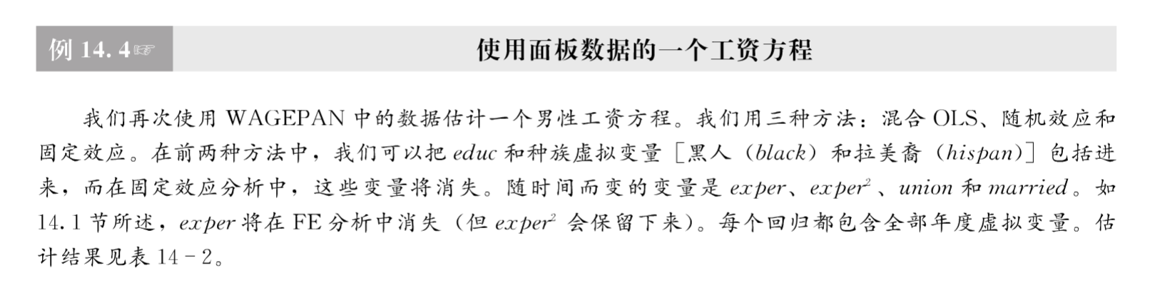
在本文中,我们以伍德里奇《计量经济学导论:现代方法》的”第14章 高级面板数据方法“的例14.4为例,使用wagepan中的数据来进行混合估计模型、随机效应模型、固定效应模型估计。
一、导入相关库
import wooldridge as woo
import statsmodels.api as sm
import pandas as pd
from linearmodels import PooledOLS,PanelOLS,RandomEffects
二、获取面板数据
wagepan = woo.dataWoo('wagepan')
#设置索引,保留数据列
wagepan = wagepan.set_index(['nr', 'year'],drop=False)
year=pd.Categorical(wagepan.year)  #将数字形式的年份转化为类别形式
wagepan['year']=year
获得数据如下所示:
               nr  year  agric  black  bus  ...  d84  d85  d86  d87  expersq
nr    year                                  ...
13    1980     13  1980      0      0    1  ...    0    0    0    0        1
      1981     13  1981      0      0    0  ...    0    0    0    0        4
      1982     13  1982      0      0    1  ...    0    0    0    0        9
      1983     13  1983      0      0    1  ...    0    0    0    0       16
      1984     13  1984      0      0    0  ...    1    0    0    0       25
          ...   ...    ...    ...  ...  ...  ...  ...  ...  ...      ...
12548 1983  12548  1983      0      0    0  ...    0    0    0    0       64
      1984  12548  1984      0      0    0  ...    1    0    0    0       81
      1985  12548  1985      0      0    0  ...    0    1    0    0      100
      1986  12548  1986      0      0    0  ...    0    0    1    0      121
      1987  12548  1987      0      0    0  ...    0    0    0    1      144

[4360 rows x 44 columns]
变量如下表所示:
| 变量 | 描述 |
|---|---|
| lwage | 工资的对数 |
| educ | 学校教育年数;不随时间变化 |
| black | 黑人取1,否则取0;不随时间变化 |
| hisp | 拉美裔取1,否则取0;不随时间变化 |
| exper | 工作年限 |
| expersq | 工作年限的平方 |
| union | 是否加入工会,加入取1,否则取0 |
| married | 已婚取1,否则取0 |
处理面板数据的模型通常有三种:混合估计模型、固定效应模型和随机效应模型。
三、混合估计模型
混合估计模型:如果从时间上看,不同个体之间不存在显著性差异;从截面上看,不同截面之间也不存在显著性差异,那么就可以直接把面板数据混合在一起用普通最小二乘估计参数。
使用所有自变量和时间虚拟变量,构建混合估计模型如下:
l
o
g
(
w
a
g
e
)
i
t
=
β
0
+
δ
0
d
8
1
t
+
.
.
.
+
δ
6
d
8
7
t
+
β
1
e
d
u
c
i
t
+
β
2
b
l
a
c
k
i
t
+
β
3
h
i
s
p
i
t
+
β
4
e
x
p
e
r
i
t
+
β
5
e
x
p
e
r
i
t
2
+
β
6
u
n
i
o
n
i
t
+
β
7
m
a
r
r
i
e
d
i
t
+
u
i
t
log(wage)_{it}=\beta_0+\delta_0d81_{t}+...+\delta_6d87_{t}+\beta_1educ_{it}\\ +\beta_2black_{it}+\beta_3hisp_{it}+\beta_4exper_{it}+\beta_5exper^2_{it}\\ +\beta_6union_{it}+\beta_7married_{it}+u_{it}
log(wage)it=β0+δ0d81t+...+δ6d87t+β1educit+β2blackit+β3hispit+β4experit+β5experit2+β6unionit+β7marriedit+uit
from linearmodels import PooledOLS
import statsmodels.api as sm

#基于数组
exog_vars = ['educ','black','hisp','exper','expersq','married','union','year']
exog = sm.add_constant(wagepan[exog_vars])
reg_pooled = PooledOLS(wagepan.lwage,exog) #创建(全部年度-1)个虚拟变量
results_pooled1 = reg_pooled.fit()
print(results_pooled1)

#基于公式
reg_pooled = PooledOLS.from_formula('lwage ~ educ + black + hisp + exper + expersq +'
            'married + union + year', data=wagepan) #创建全部年度虚拟变量
results_pooled2 = reg_pooled.fit()
print(results_pooled2)
基于数组的混合估计模型,创建(全部年度-1)个虚拟变量,返回结果:
                          PooledOLS Estimation Summary
================================================================================
Dep. Variable:                  lwage   R-squared:                        0.1893
Estimator:                  PooledOLS   R-squared (Between):              0.2066
No. Observations:                4360   R-squared (Within):               0.1692
Date:                Wed, Jul 20 2022   R-squared (Overall):              0.1893
Time:                        20:03:31   Log-likelihood                   -2982.0
Cov. Estimator:            Unadjusted
                                        F-statistic:                      72.459
Entities:                         545   P-value                           0.0000
Avg Obs:                       8.0000   Distribution:                 F(14,4345)
Min Obs:                       8.0000
Max Obs:                       8.0000   F-statistic (robust):             72.459
                                        P-value                           0.0000
Time periods:                       8   Distribution:                 F(14,4345)
Avg Obs:                       545.00
Min Obs:                       545.00
Max Obs:                       545.00

                             Parameter Estimates
==============================================================================
            Parameter  Std. Err.     T-stat    P-value    Lower CI    Upper CI
------------------------------------------------------------------------------
const          0.0921     0.0783     1.1761     0.2396     -0.0614      0.2455
educ           0.0913     0.0052     17.442     0.0000      0.0811      0.1016
black         -0.1392     0.0236    -5.9049     0.0000     -0.1855     -0.0930
hisp           0.0160     0.0208     0.7703     0.4412     -0.0248      0.0568
exper          0.0672     0.0137     4.9095     0.0000      0.0404      0.0941
expersq       -0.0024     0.0008    -2.9413     0.0033     -0.0040     -0.0008
married        0.1083     0.0157     6.8997     0.0000      0.0775      0.1390
union          0.1825     0.0172     10.635     0.0000      0.1488      0.2161
year.1981      0.0583     0.0304     1.9214     0.0548     -0.0012      0.1178
year.1982      0.0628     0.0332     1.8900     0.0588     -0.0023      0.1279
year.1983      0.0620     0.0367     1.6915     0.0908     -0.0099      0.1339
year.1984      0.0905     0.0401     2.2566     0.0241      0.0119      0.1691
year.1985      0.1092     0.0434     2.5200     0.0118      0.0243      0.1942
year.1986      0.1420     0.0464     3.0580     0.0022      0.0509      0.2330
year.1987      0.1738     0.0494     3.5165     0.0004      0.0769      0.2707
==============================================================================
基于公式的混合估计模型,创建全部年度-虚拟变量,返回结果:
                          PooledOLS Estimation Summary
================================================================================
Dep. Variable:                  lwage   R-squared:                        0.1893
Estimator:                  PooledOLS   R-squared (Between):              0.2066
No. Observations:                4360   R-squared (Within):               0.1692
Date:                Thu, Jul 21 2022   R-squared (Overall):              0.1893
Time:                        15:45:27   Log-likelihood                   -2982.0
Cov. Estimator:            Unadjusted
                                        F-statistic:                      72.459
Entities:                         545   P-value                           0.0000
Avg Obs:                       8.0000   Distribution:                 F(14,4345)
Min Obs:                       8.0000
Max Obs:                       8.0000   F-statistic (robust):             3381.6
                                        P-value                           0.0000
Time periods:                       8   Distribution:                 F(14,4345)
Avg Obs:                       545.00
Min Obs:                       545.00
Max Obs:                       545.00

                              Parameter Estimates
================================================================================
              Parameter  Std. Err.     T-stat    P-value    Lower CI    Upper CI
--------------------------------------------------------------------------------
black           -0.1392     0.0236    -5.9049     0.0000     -0.1855     -0.0930
educ             0.0913     0.0052     17.442     0.0000      0.0811      0.1016
exper            0.0672     0.0137     4.9095     0.0000      0.0404      0.0941
expersq         -0.0024     0.0008    -2.9413     0.0033     -0.0040     -0.0008
hisp             0.0160     0.0208     0.7703     0.4412     -0.0248      0.0568
married          0.1083     0.0157     6.8997     0.0000      0.0775      0.1390
union            0.1825     0.0172     10.635     0.0000      0.1488      0.2161
year[T.1980]     0.0921     0.0783     1.1761     0.2396     -0.0614      0.2455
year[T.1981]     0.1504     0.0838     1.7935     0.0730     -0.0140      0.3148
year[T.1982]     0.1548     0.0893     1.7335     0.0831     -0.0203      0.3299
year[T.1983]     0.1541     0.0944     1.6323     0.1027     -0.0310      0.3391
year[T.1984]     0.1825     0.0990     1.8437     0.0653     -0.0116      0.3766
year[T.1985]     0.2013     0.1031     1.9523     0.0510     -0.0008      0.4035
year[T.1986]     0.2340     0.1068     2.1920     0.0284      0.0247      0.4433
year[T.1987]     0.2659     0.1100     2.4166     0.0157      0.0502      0.4816
================================================================================
linearmodels的PooledOLS结果其实和statsmodels的OLS结果一致,出于完整性考虑,linearmodels加入了PooledOLS模块,我们也可以采用statsmodels的OLS模块进行估计。
import statsmodels.formula.api as smf

reg_ols = smf.ols('lwage ~ educ + black + hisp + exper + expersq +'
            'married + union + year', data=wagepan)
results_ols = reg_ols.fit()
print(results_ols.summary())
结果如下:
                            OLS Regression Results
==============================================================================
Dep. Variable:                  lwage   R-squared:                       0.189
Model:                            OLS   Adj. R-squared:                  0.187
Method:                 Least Squares   F-statistic:                     72.46
Date:                Thu, 21 Jul 2022   Prob (F-statistic):          7.25e-186
Time:                        17:08:28   Log-Likelihood:                -2982.0
No. Observations:                4360   AIC:                             5994.
Df Residuals:                    4345   BIC:                             6090.
Df Model:                          14
Covariance Type:            nonrobust
================================================================================
                   coef    std err          t      P>|t|      [0.025      0.975]
--------------------------------------------------------------------------------
Intercept        0.0921      0.078      1.176      0.240      -0.061       0.246
year[T.1981]     0.0583      0.030      1.921      0.055      -0.001       0.118
year[T.1982]     0.0628      0.033      1.890      0.059      -0.002       0.128
year[T.1983]     0.0620      0.037      1.692      0.091      -0.010       0.134
year[T.1984]     0.0905      0.040      2.257      0.024       0.012       0.169
year[T.1985]     0.1092      0.043      2.520      0.012       0.024       0.194
year[T.1986]     0.1420      0.046      3.058      0.002       0.051       0.233
year[T.1987]     0.1738      0.049      3.517      0.000       0.077       0.271
educ             0.0913      0.005     17.442      0.000       0.081       0.102
black           -0.1392      0.024     -5.905      0.000      -0.185      -0.093
hisp             0.0160      0.021      0.770      0.441      -0.025       0.057
exper            0.0672      0.014      4.909      0.000       0.040       0.094
expersq         -0.0024      0.001     -2.941      0.003      -0.004      -0.001
married          0.1083      0.016      6.900      0.000       0.077       0.139
union            0.1825      0.017     10.635      0.000       0.149       0.216
==============================================================================
Omnibus:                     1275.556   Durbin-Watson:                   0.998
Prob(Omnibus):                  0.000   Jarque-Bera (JB):            10615.542
Skew:                          -1.157   Prob(JB):                         0.00
Kurtosis:                      10.286   Cond. No.                         929.
==============================================================================

Notes:
[1] Standard Errors assume that the covariance matrix of the errors is correctly specified.
四、随机效应模型
随机效应模型实际上与混合OLS模型相同,只是它考虑了模型的结构,因此更有效。
from linearmodels import RandomEffects
import statsmodels.api as sm

#基于数组
exog_vars=['educ','black','hisp','exper','expersq','married','union','year']
exog=sm.add_constant(wagepan[exog_vars])
reg_re=RandomEffects(wagepan.lwage,exog)
results_re1=reg_re.fit()
print(results_re1)

#基于公式
reg_re = RandomEffects.from_formula('lwage ~ educ + black + hisp + exper + expersq +married + union + year', data=wagepan)
results_re2 = reg_re.fit()
print(results_re2)
基于数组的随机效应模型,创建(全部年度-1)个虚拟变量,返回结果:
                        RandomEffects Estimation Summary
================================================================================
Dep. Variable:                  lwage   R-squared:                        0.1806
Estimator:              RandomEffects   R-squared (Between):              0.1853
No. Observations:                4360   R-squared (Within):               0.1799
Date:                Thu, Jul 21 2022   R-squared (Overall):              0.1828
Time:                        16:07:49   Log-likelihood                   -1622.5
Cov. Estimator:            Unadjusted
                                        F-statistic:                      68.409
Entities:                         545   P-value                           0.0000
Avg Obs:                       8.0000   Distribution:                 F(14,4345)
Min Obs:                       8.0000
Max Obs:                       8.0000   F-statistic (robust):             68.409
                                        P-value                           0.0000
Time periods:                       8   Distribution:                 F(14,4345)
Avg Obs:                       545.00
Min Obs:                       545.00
Max Obs:                       545.00

                             Parameter Estimates
==============================================================================
            Parameter  Std. Err.     T-stat    P-value    Lower CI    Upper CI
------------------------------------------------------------------------------
const          0.0234     0.1514     0.1546     0.8771     -0.2735      0.3203
educ           0.0919     0.0107     8.5744     0.0000      0.0709      0.1129
black         -0.1394     0.0480    -2.9054     0.0037     -0.2334     -0.0453
hisp           0.0217     0.0428     0.5078     0.6116     -0.0622      0.1057
exper          0.1058     0.0154     6.8706     0.0000      0.0756      0.1361
expersq       -0.0047     0.0007    -6.8623     0.0000     -0.0061     -0.0034
married        0.0638     0.0168     3.8035     0.0001      0.0309      0.0967
union          0.1059     0.0179     5.9289     0.0000      0.0709      0.1409
year.1981      0.0404     0.0247     1.6362     0.1019     -0.0080      0.0889
year.1982      0.0309     0.0324     0.9519     0.3412     -0.0327      0.0944
year.1983      0.0202     0.0417     0.4840     0.6284     -0.0616      0.1020
year.1984      0.0430     0.0515     0.8350     0.4037     -0.0580      0.1440
year.1985      0.0577     0.0615     0.9383     0.3482     -0.0629      0.1782
year.1986      0.0918     0.0716     1.2834     0.1994     -0.0485      0.2321
year.1987      0.1348     0.0817     1.6504     0.0989     -0.0253      0.2950
==============================================================================
基于公式的随机效应模型,创建全部年度虚拟变量,返回结果:
                        RandomEffects Estimation Summary
================================================================================
Dep. Variable:                  lwage   R-squared:                        0.1806
Estimator:              RandomEffects   R-squared (Between):              0.1853
No. Observations:                4360   R-squared (Within):               0.1799
Date:                Thu, Jul 21 2022   R-squared (Overall):              0.1828
Time:                        16:07:49   Log-likelihood                   -1622.5
Cov. Estimator:            Unadjusted
                                        F-statistic:                      68.409
Entities:                         545   P-value                           0.0000
Avg Obs:                       8.0000   Distribution:                 F(14,4345)
Min Obs:                       8.0000
Max Obs:                       8.0000   F-statistic (robust):             846.19
                                        P-value                           0.0000
Time periods:                       8   Distribution:                 F(14,4345)
Avg Obs:                       545.00
Min Obs:                       545.00
Max Obs:                       545.00

                              Parameter Estimates
================================================================================
              Parameter  Std. Err.     T-stat    P-value    Lower CI    Upper CI
--------------------------------------------------------------------------------
black           -0.1394     0.0480    -2.9054     0.0037     -0.2334     -0.0453
educ             0.0919     0.0107     8.5744     0.0000      0.0709      0.1129
exper            0.1058     0.0154     6.8706     0.0000      0.0756      0.1361
expersq         -0.0047     0.0007    -6.8623     0.0000     -0.0061     -0.0034
hisp             0.0217     0.0428     0.5078     0.6116     -0.0622      0.1057
married          0.0638     0.0168     3.8035     0.0001      0.0309      0.0967
union            0.1059     0.0179     5.9289     0.0000      0.0709      0.1409
year[T.1980]     0.0234     0.1514     0.1546     0.8771     -0.2735      0.3203
year[T.1981]     0.0638     0.1601     0.3988     0.6901     -0.2500      0.3777
year[T.1982]     0.0543     0.1690     0.3211     0.7481     -0.2770      0.3856
year[T.1983]     0.0436     0.1780     0.2450     0.8065     -0.3054      0.3926
year[T.1984]     0.0664     0.1871     0.3551     0.7225     -0.3003      0.4332
year[T.1985]     0.0811     0.1961     0.4136     0.6792     -0.3034      0.4656
year[T.1986]     0.1152     0.2052     0.5617     0.5744     -0.2870      0.5175
year[T.1987]     0.1583     0.2143     0.7386     0.4602     -0.2618      0.5783
================================================================================
五、固定效应模型
在linearmodels中固定效应分析使用PanelOLS工具。
当使用个体固定效应时,不随时间变化的变量应该从模型中剔除,因此剔除educ、black、hisp等三个变量。同时,由于模型中加入了年度虚拟变量,变量exper也应该排除,否则会出现多重共线性。
from linearmodels import PanelOLS

#基于数组
exog_vars=['expersq','married','union','year']
exog=wagepan[exog_vars]
reg_fe=PanelOLS(wagepan.lwage,exog,entity_effects=True)
results_fe1=reg_fe.fit()
print(results_fe1)

#基于公式
reg_fe = PanelOLS.from_formula('lwage ~ expersq+ married + union + year + EntityEffects', data=wagepan)
results_fe2 = reg_fe.fit()
print(results_fe2)
基于数组的固定效应模型,创建(全部年度-1)个虚拟变量,返回结果:
                          PanelOLS Estimation Summary
================================================================================
Dep. Variable:                  lwage   R-squared:                        0.1806
Estimator:                   PanelOLS   R-squared (Between):              0.2386
No. Observations:                4360   R-squared (Within):               0.1806
Date:                Thu, Jul 21 2022   R-squared (Overall):              0.2361
Time:                        16:46:25   Log-likelihood                   -1324.8
Cov. Estimator:            Unadjusted
                                        F-statistic:                      83.851
Entities:                         545   P-value                           0.0000
Avg Obs:                       8.0000   Distribution:                 F(10,3805)
Min Obs:                       8.0000
Max Obs:                       8.0000   F-statistic (robust):             83.851
                                        P-value                           0.0000
Time periods:                       8   Distribution:                 F(10,3805)
Avg Obs:                       545.00
Min Obs:                       545.00
Max Obs:                       545.00

                             Parameter Estimates
==============================================================================
            Parameter  Std. Err.     T-stat    P-value    Lower CI    Upper CI
------------------------------------------------------------------------------
expersq       -0.0052     0.0007    -7.3612     0.0000     -0.0066     -0.0038
married        0.0467     0.0183     2.5494     0.0108      0.0108      0.0826
union          0.0800     0.0193     4.1430     0.0000      0.0421      0.1179
year.1981      0.1512     0.0219     6.8883     0.0000      0.1082      0.1942
year.1982      0.2530     0.0244     10.360     0.0000      0.2051      0.3008
year.1983      0.3544     0.0292     12.121     0.0000      0.2971      0.4118
year.1984      0.4901     0.0362     13.529     0.0000      0.4191      0.5611
year.1985      0.6175     0.0452     13.648     0.0000      0.5288      0.7062
year.1986      0.7655     0.0561     13.638     0.0000      0.6555      0.8755
year.1987      0.9250     0.0688     13.450     0.0000      0.7902      1.0599
==============================================================================

F-test for Poolability: 9.1568
P-value: 0.0000
Distribution: F(544,3805)

Included effects: Entity
基于公式的固定效应模型,创建全部年度虚拟变量,返回结果:
                          PanelOLS Estimation Summary
================================================================================
Dep. Variable:                  lwage   R-squared:                        0.1806
Estimator:                   PanelOLS   R-squared (Between):             -0.0052
No. Observations:                4360   R-squared (Within):               0.1806
Date:                Thu, Jul 21 2022   R-squared (Overall):              0.0807
Time:                        16:47:26   Log-likelihood                   -1324.8
Cov. Estimator:            Unadjusted
                                        F-statistic:                      83.851
Entities:                         545   P-value                           0.0000
Avg Obs:                       8.0000   Distribution:                 F(10,3805)
Min Obs:                       8.0000
Max Obs:                       8.0000   F-statistic (robust):             8850.2
                                        P-value                           0.0000
Time periods:                       8   Distribution:                 F(10,3805)
Avg Obs:                       545.00
Min Obs:                       545.00
Max Obs:                       545.00

                              Parameter Estimates
================================================================================
              Parameter  Std. Err.     T-stat    P-value    Lower CI    Upper CI
--------------------------------------------------------------------------------
expersq         -0.0052     0.0007    -7.3612     0.0000     -0.0066     -0.0038
married          0.0467     0.0183     2.5494     0.0108      0.0108      0.0826
union            0.0800     0.0193     4.1430     0.0000      0.0421      0.1179
year[T.1980]     1.4260     0.0183     77.748     0.0000      1.3901      1.4620
year[T.1981]     1.5772     0.0216     72.966     0.0000      1.5348      1.6196
year[T.1982]     1.6790     0.0265     63.258     0.0000      1.6270      1.7310
year[T.1983]     1.7805     0.0333     53.439     0.0000      1.7151      1.8458
year[T.1984]     1.9161     0.0417     45.982     0.0000      1.8344      1.9978
year[T.1985]     2.0435     0.0515     39.646     0.0000      1.9424      2.1446
year[T.1986]     2.1915     0.0630     34.771     0.0000      2.0679      2.3151
year[T.1987]     2.3510     0.0762     30.867     0.0000      2.2017      2.5004
================================================================================

F-test for Poolability: 9.1568
P-value: 0.0000
Distribution: F(544,3805)

Included effects: Entity
创建年度虚拟变量的其他方式:
#引入时间虚拟变量的个体固定效应:基于数组
year_cat = pd.Categorical(wagepan.year) #将数字形式的年份转化为类别形式
wagepan['year_cat'] = year_cat
exog_vars =['expersq','married','union','year_cat']
exog = wagepan[exog_vars]
res_fe = PanelOLS(wagepan['lwage'], exog, entity_effects=True) #包含(全部年度-1)个虚拟变量
results_fe = res_fe.fit()
print(results_fe)

#引入时间虚拟变量的个体固定效应:基于公式
wagepan['y81'] = (wagepan['year'] == 1981).astype(int)  # False=0, True=1
wagepan['y82'] = (wagepan['year'] == 1982).astype(int)
wagepan['y83'] = (wagepan['year'] == 1983).astype(int)
wagepan['y84'] = (wagepan['year'] == 1984).astype(int)
wagepan['y85'] = (wagepan['year'] == 1985).astype(int)
wagepan['y86'] = (wagepan['year'] == 1986).astype(int)
wagepan['y87'] = (wagepan['year'] == 1987).astype(int)
reg_dum = PanelOLS.from_formula('lwage ~ expersq+ married + union + y81 + y82'
                               '+ y83 + y84 + y85 + y86 + y87 + EntityEffects',                                     data=wagepan)
results_dum = reg_dum.fit()
print(results_dum)

#引入时间虚拟变量的个体固定效应:基于公式
wagepan= pd.get_dummies(data=wagepan, columns=['year'])
reg_dum = PanelOLS.from_formula('lwage ~ expersq+ married + union +year_1981+'
                               'year_1982 +year_1983+year_1984+year_1985+year_1986+'
                                'year_1987+EntityEffects', data=wagepan)
results_dum = reg_dum.fit()
print(results_dum)
六、模型比较
linearmodels提供了模型结果比较工具compare,我们可以通过语句from linearmodels import compare载入模型比较工具,我们对基于数组的混合估计模型、随机效应模型、固定效应模型进行比较。
from linearmodels.panel import compare
print(compare({'Pooled':results_pooled1,'RE':results_re1,'FE':results_fe1}))
结果如下:
                            Model Comparison
=======================================================================
                                Pooled                RE             FE
-----------------------------------------------------------------------
Dep. Variable                    lwage             lwage          lwage
Estimator                    PooledOLS     RandomEffects       PanelOLS
No. Observations                  4360              4360           4360
Cov. Est.                   Unadjusted        Unadjusted     Unadjusted
R-squared                       0.1893            0.1806         0.1806
R-Squared (Within)              0.1692            0.1799         0.1806
R-Squared (Between)             0.2066            0.1853         0.2386
R-Squared (Overall)             0.1893            0.1828         0.2361
F-statistic                     72.459            68.409         83.851
P-value (F-stat)                0.0000            0.0000         0.0000
=====================     ============   ===============   ============
const                           0.0921            0.0234
                              (1.1761)          (0.1546)
educ                            0.0913            0.0919
                              (17.442)          (8.5744)
black                          -0.1392           -0.1394
                             (-5.9049)         (-2.9054)
hisp                            0.0160            0.0217
                              (0.7703)          (0.5078)
exper                           0.0672            0.1058
                              (4.9095)          (6.8706)
expersq                        -0.0024           -0.0047        -0.0052
                             (-2.9413)         (-6.8623)      (-7.3612)
married                         0.1083            0.0638         0.0467
                              (6.8997)          (3.8035)       (2.5494)
union                           0.1825            0.1059         0.0800
                              (10.635)          (5.9289)       (4.1430)
year.1981                       0.0583            0.0404         0.1512
                              (1.9214)          (1.6362)       (6.8883)
year.1982                       0.0628            0.0309         0.2530
                              (1.8900)          (0.9519)       (10.360)
year.1983                       0.0620            0.0202         0.3544
                              (1.6915)          (0.4840)       (12.121)
year.1984                       0.0905            0.0430         0.4901
                              (2.2566)          (0.8350)       (13.529)
year.1985                       0.1092            0.0577         0.6175
                              (2.5200)          (0.9383)       (13.648)
year.1986                       0.1420            0.0918         0.7655
                              (3.0580)          (1.2834)       (13.638)
year.1987                       0.1738            0.1348         0.9250
                              (3.5165)          (1.6504)       (13.450)
======================= ============== ================= ==============
Effects                                                          Entity
-----------------------------------------------------------------------

T-stats reported in parentheses
参考资料:
https://bashtage.github.io/linearmodels/panel/examples/using-formulas.html


 1万+
1万+


 被折叠的 条评论
为什么被折叠?
被折叠的 条评论
为什么被折叠?
 到【灌水乐园】发言


