Turbo-Plonk：用于特定SNARK程序的语法提案

1. 引言

Aztec protocol 团队的Gabizon 和 Williamson 发表于2020年ZKProof第3届Workshop的论文《Proposal: The Turbo-PLONK program syntax for specifying SNARK programs》。

代码实现有：

• https://github.com/AZTECProtocol/barretenberg

近期的Marlin和PLONK都是依赖于Polynomial commitment scheme来构建zk-SNARK了，而与待证明的statement采用R1CS constraints 关系并不紧密。主要原因在于，polynomial commitment scheme构建zk-SNARK中，其verifier equation 为checked “in the clear” on a random opening of the prover polynomials，而之前的R1CS constraint zk-SNARK方案中的verifier equation 是“in the exponent” using a pairing。

在本论文中，提供了一种框架来实现更通用和灵活的constraint类型，该框架称为 turbo-PLONK programs。

turbo-PLONK programs 框架可提供：

• fixed-base elliptic curve scalar multiplication (仅需1 turbo-PLONK gate for each two input bits)
• a primitive useful for constructing Pedersen hashes。

同时，使用Grumkin curve (255-bit curve embedded over bn254)，针对scalar multiplication操作，本文的方案相比于Groth16快约2倍。

2. Turbo PLONK programs

a turbo-PLONK program $\mathcal{P}$ 可看成是一系列的状态$v\in {\mathbb{F}}^w$，其中$w$为state size，由program designer设定。
Proof size和Prover run time随着$w$线性增加，通常$w$的值为3或者4。

$\mathcal{P}$支持两种类型：

• transition gate
• copy constraint

相应的valid execution trace 为 $T\in ({\mathbb{F}}^w{)}^t$。

2.1 transition gate

$\mathcal{P}$ 的 transition constraint 对应为 a $2w+l$-variate degree at most $d$ polynomial $P$，其中$d$为$\mathcal{P}$的degree，建议设置$d=w+1$，$l$为the selector number。

$\mathcal{P}$ 的 transition gate 中包含了：

• 所有的transition constraints
• $l$ selector vectors $q_1,\cdots ,q_l\in {\mathbb{F}}^t$

若满足以下条件，可称$T$ satisfy the transition gate：

• 对于每一个transition constraint $i\in [t]$，$P(T_{i,1},\cdots ,T_{i,w},T_{i+1,1},\cdots ,T_{i+1,w},q_1(i),\cdots ,q_l(i))=0$均成立。

2.2 copy constraint

a partition of $w\times t$ into distinct sets { S i } \{S_i\} {Si​}。

若满足以下条件，可称$T$ satisfy the copy constraint：

• 当$(i,j)和(i^{\prime },j^{\prime })$ 属于partition中的同一set时，有$T_{i,j}=T_{i^{\prime },j^{\prime }}$。

copy constraint可理解为enabling memory access，因为我们可以要求execution trace中的后一值等于前一值。

3. arithmetic circuit的特例

arithmetic circuit的表达规则为：

• 每一行表示1个gate；
• 每一行中的值（row values）表示该gate对应的incoming wire values和outgoing wire values
• 若需表达 fan-in $t$ circuits，则设置$w=t+1$。

如，对于 fan-in $2$，其row values 为$v_1,v_2,v_3$，分别为该row 对应gate的left wire value、right wire value 和 output wire value。

3.1 transition constraint

对于transition constraint，其不会用到下一行的values $T_{i+1,1},\cdots ,T_{i+1,w}$，transition constraint仅check 其所在行中的值是否符合addition gate或multiplication gate规则。可借助 3个selectors 和 1个constraint polynomial $P$ of degree $t+1$。
如对于fan-in $2$ circuit，可定义为：
$P(q_L,q_R,q_M,x_1,x_2,x_3)=q_L\cdot x_1+q_R\cdot x_2+q_M\cdot x_1{x}_2-x_3$

具体为：

• 对于addition gate，设置$q_L(i)=q_R(i)=1,q_M(i)=0$；
• 对于multiplication gate，设置$q_L(i)=q_R(i)=0,q_M(i)=1$。

3.2 copy constraint

copy constraint用于enforce the wiring of the circuit。如，对于4th gate，其left wire 为 the second gate的output wire，则可表示为：
$T_{2,3}=T_{4,1}$

4. 基础技术

Turbo-PLONK中主要使用了2个基础技术：

• Look Ups
• Interleaving PLONK Gates

4.1 Look Ups

假设有2个selector $q_1,q_2$，为了enforce：
row $i$的第一个值 等于 $q_b(i)$，其中$b$为同一行中的第二个值。

则相应的constraint可表示为：【即$x_1=q_{x_2}$。当$x_2$等于1时，有$x_1=q_1$；当$x_2=2$时，有$x_1=q_2$。】
$x_1=-q_1\cdot (x_2-2)+q_2\cdot (x_2-1)$

接下来，如果需要在两个值之间进行选择，或者选择其负数，可引入row中的第三个值，设其为$1$或$-1$，相应的constraint可表示为：【即$x_1=x_3\cdot q_{x_2}$。其中$x_3$取$1$或$-1$。】
$x_1=(-q_1\cdot (x_2-2)+q_2\cdot (x_2-1))\cdot x_3$

4.2 Interleaving PLONK Gates

之前设计的transition gate对应为a set of $2w+l$-variate polynomials，伴随有$l$个selector polynomials。
针对每一行，可专门设计不同的subset of constraints depending on the row。

如，已知2个gate $G_1,G_2$，需仅对$G_1$ enforce some row transitions，而仅对$G_2$ enforce 另一组row transitions，$G_1$和$G_2$之间有一些共同的constraints。

通用的解决方案为：增加2个selector $q_{G_1},q_{G_2}$，根据指定row中相应的gate是否激活对应取值为$0或1$。然后multiply each constraint $P$ in $G_i$ by $q_{G_i}$。同时，defIne the new gate’s constraints to be the union of these constraints from both gates。

5. Fixed-base scalar multiplication

在椭圆密码学中，最贵的操作之一就是scalar multiplication：

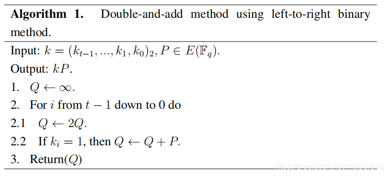
假设scalar $k=15$，对应的二进制表示为$0b1111$，即$k$的hamming weight为4。若采用如上double-and-add算法，需要3次point doubling操作和4次point addtion操作，整个操作的复杂度高度依赖于the number of set 或 hamming weight，且加法操作仅在当前bit不为0时执行。

为了减少scalar multiplication操作的计算复杂度，方法之一是reduce hamming weights of the scalar。

假设$\#E({\mathbb{F}}_q)=rh$，其中$r$为prime的，$h$很小，使得$r\approx q$。point $P和Q$均具有order $r$，scalar $k$为在$[1,r-1]$区间的随机值。
$k$的二进制表示为$(k_{t-1},\cdots ,k_2,k_1,k_0{)}_2$，其中$t\approx m=\lceil {\log }_{2}q\rceil$。若point $P$为fixed且storage is availabe，则point multilication 可借助pre-computation table来加速。
具体的加速方法有：【本节主要关注fixed-base下对hamming weight的reduce。】

• Non-Adjacent Form（NAF）
• Window Method
• Zero Occurence Evaluation
• Lim and Lee’s Method
• Tsaur and Chou’s Method
• Direct Doubling Method
• Mohamed, Hashim and Hutter’s Method

本文主要关注NAF算法：
若$P=(x,y)\in E({\mathbb{F}}_q)$，则$-P$表示为$-P=(x,-y)$。因此，point减法 可转换为 point加法 进行运算。

针对NAF的主要优化策略为：

• 1）约定 scalar $s$ NAF representation；
• 2）选择每轮中要add的correction point；
• 3）add the selected point；
• 4）initialization gate

5.1 the NAF scalar representation

假设scalar $s$的取值范围为 { 1 , . . , M } \{1,..,M\} {1,..,M}，其中$M<r/2$，且存在整数$n$使得$M=2\cdot 4^n-1$。
此时，$s$可表示为$s=t+{\sum }_{i=0}^{n-1}{b}_i\cdot 4^i$，其中 b i ∈ { − 3 , − 1 , 1 , 3 } , t ∈ { 4 n , 4 n + 1 } b_i\in\{-3,-1,1,3\},t\in\{4^n,4^n+1\} bi​∈{−3,−1,1,3},t∈{4n,4n+1}。可将$s$看成是由$n$个input quads { b i } \{b_i\} {bi​} 和 1个input bit $t$组成。

Turbo-Plonk的program针对此情况，包含了$n$轮运算，设置初始 $sum$ 为 $t[g]$ ，在第$i$轮：

• 为add { − 3 [ g i ] , − 1 [ g i ] , 1 [ g i ] , 3 [ g i ] } \{-3[g_i],-1[g_i],1[g_i],3[g_i]\} {−3[gi​],−1[gi​],1[gi​],3[gi​]} 中之一，其中$g_i=4^{n-i}[g]$ 为 a precomputed power of our actual generator。

为了reduce program width，优化策略为：

• only explicitly represent “intermediate sums” of our scalar, and not the actual input quads。原因为：the intermediate sums are more convenient than the quads in checking the correct scalar $s$ was used。

intermediate sums的定义为：

• $a_0=t/4^n,a_1=t/4^{n-1}+b_{n-1}$，对于 i ∈ { 2 , ⋯   , n } i\in \{2,\cdots,n\} i∈{2,⋯,n}，有$a_i=4\cdot a_{i-1}+b_{n-i}$

最终有$a_n=s$。

为了cancel the effect of the sign of the input quad，优化策略为：

• squaring the difference of two intermediate sums，因为 the $x$ coordinate of the point we want to select only depends on the magnitude on the difference。（而若想explicityly represent this magnitude，将再次增加the width of the final program。）

对于2-bit NAF addition gate，对应为 已知 row values $(x_1,y_1,x_{\alpha ,1},a_{i-1}),(x_2,y_2,x_{\alpha ,2},a_i)$，需定义a width 4 program来 check：

• $(x_2,y_2)=(x_1,y_1)+(a_i-4a_{i-1})[g_i]$

5.2 selecting the correct point to add

1）第一步为采用4.1节中的lookup方法，来选择特定round中需add的coordinates of the correct point。
以round $i\in [n]$为例，定义 $g_i=(x_{\beta },y_{\beta }),3[g_i]=(x_{\gamma },y_{\gamma })$。
$(x_{\alpha },y_{\alpha })$为在该轮中需add到input中的point。因此，$(x_{\alpha },y_{\alpha })$ 为 { ( x β , y β ) , ( x β , − y β ) , ( x γ , y γ ) , ( x γ , − y γ ) } \{(x_{\beta},y_{\beta}),(x_{\beta},-y_{\beta}),(x_{\gamma},y_{\gamma}),(x_{\gamma},-y_{\gamma})\} {(xβ​,yβ​),(xβ​,−yβ​),(xγ​,yγ​),(xγ​,−yγ​)} set 中的一个point。

$x_{\alpha }$可通过以下方式恢复：
$\frac{(a_i-4a_{i-1}{)}^2-9}{-8}{x}_{\beta }+\frac{(a_i-4a_{i-1}{)}^2-1}{8}{x}_{\gamma }=x_{\alpha }\Rightarrow (a_i-4a_{i-1}{)}^2\frac{x_{\gamma }-x_{\beta }}{8}+\frac{9x_{\beta }-x_{\gamma }}{8}=x_{\alpha }$

替换其中的precomputed constants为selectors：
$q_{x_{\alpha ,1}}=\frac{x_{\gamma }-x_{\beta }}{8},q_{x_{\alpha ,2}}=\frac{x_{\gamma }-x_{\beta }}{8}\Rightarrow (a_i-4a_{i-1}{)}^2{q}_{x_{\alpha ,1}}+q_{x_{\alpha ,2}}=x_{\alpha }$

将$x_{\alpha }$存储为distinct wire value，跟使用cubic polynomial identity来提取相应的$y$坐标 $y_{\alpha }$：
$\frac{(x_{\alpha }-x_{\gamma })(a_i-4a_{i-1})}{(x_{\beta }-x_{\gamma })}{y}_{\beta }+\frac{(x_{\alpha }-x_{\beta })(a_i-4a_{i-1})}{3(x_{\gamma }-x_{\beta })}{y}_{\gamma }=y_{\alpha }$
$\Rightarrow (x_{\alpha }\frac{3y_{\beta }-y_{\gamma }}{3(x_{\beta }-x_{\gamma })}+\frac{x_{\beta }{y}_{\gamma }-3x_{\gamma }{y}_{\beta }}{3(x_{\beta }-x_{\gamma })})(a_i-4a_{i-1})=y_{\alpha }$

引入2个precomputed selectors，表示为：
$q_{y_{\alpha ,1}}=\frac{3y_{\beta }-y_{\gamma }}{3(x_{\beta }-x_{\gamma })},q_{y_{\alpha ,2}}=\frac{x_{\beta }{y}_{\gamma }-3x_{\gamma }{y}_{\beta }}{3(x_{\beta }-x_{\gamma })}$
$\Rightarrow (x_{\alpha }{q}_{y_{\alpha ,1}}+q_{y_{\alpha ,2}})(a_i-4a_{i-1})=y_{\alpha }$

可将$y_{\alpha }^2$表示为$x_{\alpha }^3+b_{curve}$，其中$b_{curve}$为short weierstrass curve参数。对于BN254 embedded curve，$b_{curve}=-17$。

5.3 add the selected point

在5.2节，实现了select the correct point to add in a given round，在本节，将讲述如何actually add the selected point。

在每一轮，当add powers of disjoint magnitude of generator时，可使用不处理重复$x$坐标值的incomplete affine addtion公式，如，对于$(x_1,y_1)+(x_{\alpha },y_{\alpha })=(x_2,y_2)$，相应可表示为：
$x_2=(\frac{y_{\alpha }-y_1}{x_{\alpha }-x_1}{)}^2-x_{\alpha }-x_1$
$y_2=(\frac{y_{\alpha }-y_1}{x_{\alpha }-x_1}{)}^2(x_1-x_2)-y_1$

对此，可以identity表示通过gate来evaluate，即：
$(x_2+x_{\alpha }+x_1)(x_{\alpha }-x_1{)}^2-(y_{\alpha }-y_1{)}^2=0$
$(y_2+y_1)(x_{\alpha }-x_1)-(y_{\alpha }-y_1)(x_1-x_2)=0$

借助5.2节的precomputed selectors，以上$x$和$y$坐标 check可转换为：
$(x_2+x_{\alpha }+x_1)(x_{\alpha }-x_1{)}^2+2(a_i-4a_{i-1})(x_{\alpha }{q}_{y_{\alpha ,1}}+q_{y_{\alpha ,2}})y_1-y_1^2-b_{curve}=0$
$(y_2+y_1)(x_{\alpha }-x_1)-((a_i-4a_{i-1})(x_{\alpha }{q}_{y_{\alpha ,1}}+q_{y_{\alpha ,2}})-y_1)(x_1-x_2)=0$

5.4 initialization gate

最后，还需要add 5.1节的offset $t$，实现过程为：

• 根据$a_0=1$还是$a_0=1+1/4^n$，将$(x_0,y_0)$分别初始化为$(4^n)[g]$或者$(4^n+1)[g]$。
• 采用degree two constraint来验证相应的$a_0$是否在指定区间内。

最终，将整个fixed-base scalar multiplication 以 $n+1$ 行 2-bit NAF addtion gate表示为：
$\left(\begin{array}{cccc}{x}_0& y_0& x_{\alpha ,0}& a_0\\ x_1& y_1& x_{\alpha ,1}& a_1\\ ⋮& ⋮& ⋮& ⋮\\ x_n& y_n& x_{\alpha ,n}& a_n\end{array}\right)$

具体见https://github.com/AZTECProtocol/barretenberg中的 create_fixed_group_add_gate() 和 create_fixed_group_add_gate_with_init() 函数实现。

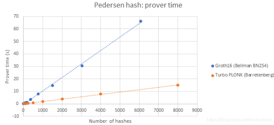
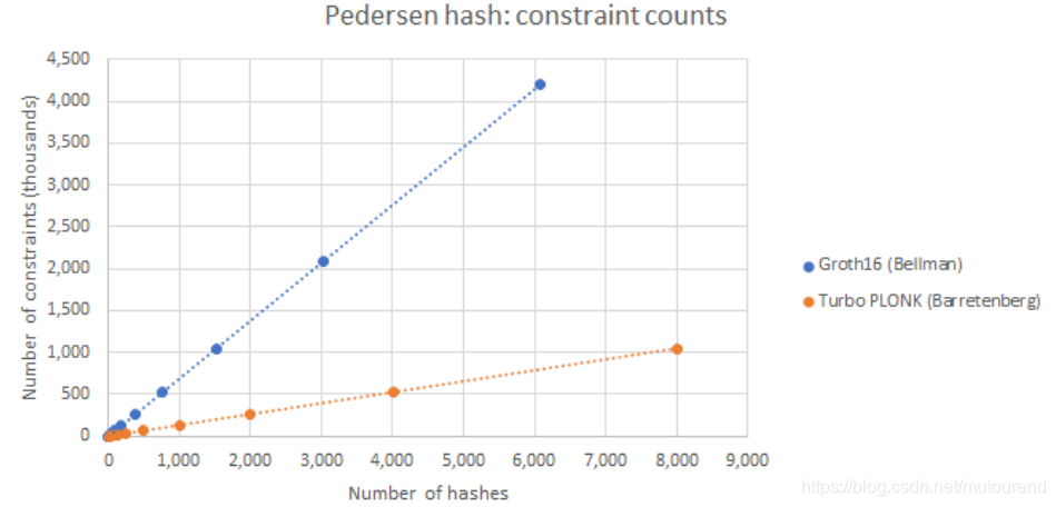
6. BN254 curve Pedersen hash 性能评估

基于BN254 curve 将Groth16中的Pedersen hash （Bellman）Prove 时间 与 barretenberg 中的TurboPLONK 实现对比，TuroPLONK的速度快将近5倍，且TurboPLONK中的constraints数量 比 Groth16中的R1CS constraints数量 少 将近5倍：【但是，单个TuboPLONK constraint的prove计算量 约为 单个Groth16 constraint prove计算量的2倍。而且，Groth16中20%的constraint都需要bit decomposition。TurboPLONK中这些binary gate的prove time 要比 Groth16中的 贵4倍左右。（由于TurboPLONK中不需要判断 the scalars in prover computation are actually equal to the witness。）】

从multi-scalar-multiplication over elliptic curves的维度看，就 Libff、Bellman、Barretenberg 这三个库的实现，性能对比为：【multi-scalar-multiplication in $G_1$】

Barretenberg 在普通消费者硬件上，执行100万次scalar multiplication运算的时间小于1秒。

7. different-base scalar multiplication

Pippenger’s multi-exponentiation 是当前计算multiple scalar-multiplication over different bases 最快的算法。

本文发现，当计算multi-products时，“使用affine坐标系的point addtion 公式” 比 “使用projective坐标系和jacobian坐标系的point addition 公式” 所需的field multiplication数量更少。

当采用affine坐标系时，相应的point addition公式为：
$\lambda =\frac{y_2-y_1}{x_2-x_1}\mathrm{m}\mathrm{o}\mathrm{d}p$
$x_3={\lambda }^2-(x_2+x_1)\mathrm{m}\mathrm{o}\mathrm{d}p$
$y_3=\lambda (x_1-x_3)-y_1\mathrm{m}\mathrm{o}\mathrm{d}p$

计算$\lambda$需要一个 modular inverse运算，其比单个的field multiplication运算贵一个数量级。

但是，Pippenger multi-product可生成sequences of independent point additions。即，the outputs of additions in the sequence are not inputs to any additions in sequence。

因此，可使用Montgomery’s trick来计算batch modular inverses：
∀ i ∈ { 1 , ⋯   , n } : d i = ∏ j = 1 i − 1 a j \forall i\in\{1,\cdots,n\}: d_i=\prod_{j=1}^{i-1}a_j ∀i∈{1,⋯,n}:di​=∏j=1i−1​aj​
$s=(d_n{a}_n{)}^{-1}$
∀ i ∈ { 1 , ⋯   , n } : e i = s ∏ j = i + 1 n a j \forall i\in\{1,\cdots,n\}:e_i=s\prod_{j=i+1}^{n}a_j ∀i∈{1,⋯,n}:ei​=s∏j=i+1n​aj​
∀ i ∈ { 1 , ⋯   , n } : r i = d i e i \forall i\in\{1,\cdots,n\}:r_i=d_ie_i ∀i∈{1,⋯,n}:ri​=di​ei​

假设有足够大的$n$，则batch modular inverse的计算量为：3 field multiplications per inverse。affine坐标系下，整个计算point addition的计算量为 6个field multiplication。
而projective坐标系下，对于short Weierstrass curve，其传统的mixed-addition需要 11个field multiplication。

参考资料

[1] 2020年论文 Proposal: The Turbo-PLONK program syntax for specifying SNARK programs
[2] 2013年论文 Fixed-Base Comb with Window-Non-Adjacent Form (NAF) Method for Scalar Multiplication