


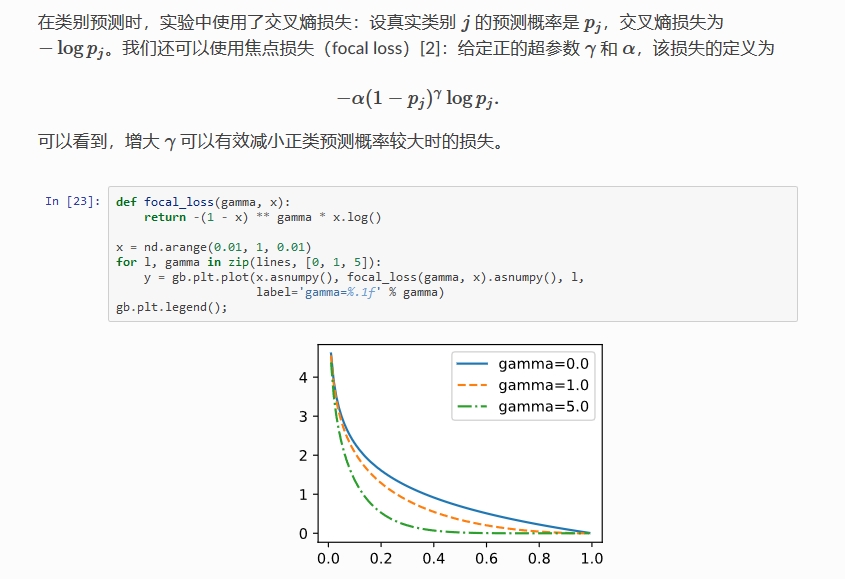
文章目录
一、目标检测中的分类损失
-
softmax_cross_entropy_loss(多分类)以及sigmoid_cross_entropy_loss(二分类)可参考博客: TensorFLow 中的损失函数 -
Focal loss(全局视角):- 思想:用一个权重条件函数(置信度的角度)去降低
易分样本(inference 中概率得分较大的)对损失的贡献(得分较大时降低其损失值,使得简单样本对损失的影响更小) - 使用场景:解决 one-stage 的目标检测中背景样本和前景样本的不平衡问题
- 调参经验:
- 降低 neg_overlap 的值(eg:0.3),ignore 一部分(0.3~0.5)label noise sample(1、标签打错了,2、困难样本)
- fine-tuning 时用:先在原始 loss 上预训练几个 epoch,然后再换成 focal loss
- 增加 anchor 数量、batch_size 等
- 分类 loss 选择
LOGISTIC(二分类)而不是SOFTMAX(多分类)
- 思想:用一个权重条件函数(置信度的角度)去降低
-
Focal loss 公式:-
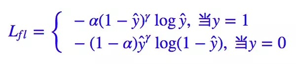
多分类公式: F L ( p t ) = − α t ( 1 − p t ) γ l o g ( p t ) FL(p_t) = -\alpha_t(1 - p_t)^{\gamma} log(p_t) FL(pt)=−αt(1−pt)γlog(pt)
-
α
t
\alpha_t
αt:控制类别间的权重比例,例如二分类中的 0.25(
pos:neg = 1:3) - γ \gamma γ:控制 loss 衰减的快慢,结合 ( 1 − p t ) (1 - p_t) (1−pt) 解决难易样本不平衡的问题
- 参数组合:论文中效果较好的为
α
=
0.25
,
γ
=
2.0
\alpha = 0.25,\gamma=2.0
α=0.25,γ=2.0
-
α
t
\alpha_t
αt:控制类别间的权重比例,例如二分类中的 0.25(
-
二分类公式及 pytorch 代码实现:
- 二分类公式
- pytorch 代码实现(
mmdetection:mmdet/models/losses/focal_loss.py):def py_sigmoid_focal_loss(pred, target, weight=None, gamma=2.0, alpha=0.25, reduction='mean', avg_factor=None): pred_sigmoid = pred.sigmoid() target = target.type_as(pred) pt = (1 - pred_sigmoid) * target + pred_sigmoid * (1 - target) focal_weight = (alpha * target + (1 - alpha) * (1 - target)) * pt.pow(gamma) loss = F.binary_cross_entropy_with_logits( pred, target, reduction='none') * focal_weight loss = weight_reduce_loss(loss, weight, reduction, avg_factor) return loss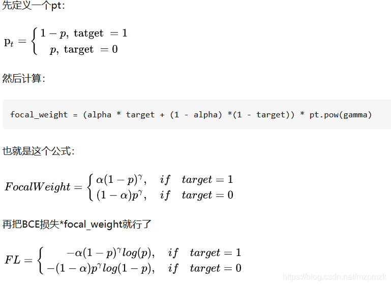
- 二分类公式
-
-
caffe 中的实现,参见 https://github.com/chuanqi305/FocalLoss
layer { name: "mbox_loss" type: "MultiBoxFocalLoss" // change the type bottom: "mbox_loc" bottom: "mbox_conf" bottom: "mbox_priorbox" bottom: "label" top: "mbox_loss" include { phase: TRAIN } propagate_down: true propagate_down: true propagate_down: false propagate_down: false loss_param { normalization: VALID } focal_loss_param { alpha: 0.25 gamma: 2.0 } multibox_loss_param { loc_loss_type: SMOOTH_L1 conf_loss_type: SOFTMAX // 二分类的时候换成 LOGISTIC 效果会好些 loc_weight: 1.0 num_classes: 21 share_location: true match_type: PER_PREDICTION overlap_threshold: 0.5 use_prior_for_matching: true background_label_id: 0 use_difficult_gt: true neg_pos_ratio: 3.0 neg_overlap: 0.5 code_type: CENTER_SIZE ignore_cross_boundary_bbox: false mining_type: NONE #do not use OHEM } } -
one-stage detector 精度比不上 two-stage detector 的原因:
- 正负样本比例极度不平衡(一般大约 10000:1),且绝大部分负样本都是 easy example
gradient 被 easy example dominant,往往这些 easy example 虽然 loss 很低,但由于数量众多,对于 loss 依旧有很大贡献,从而导致收敛到不够好的一个结果- 若分类器无脑地把所有 bbox 统一归类为 background,accuracy 也可以刷得很高。于是乎,分类器的训练就失败了。分类器训练失败,检测精度自然就低了
- two-stage 系有 RPN 罩着,RPN 会对 anchor 进行简单的二分类,anchor box 数量降低很多(1~2k),后续再使用 OHEM+按 class 比例 sample(eg:1:3),即可很好的进行训练
-
OHEM+按 class 比例 sample 原理:
- each example is scored by its loss, non-maximum suppression (nms) is then applied, and a minibatch is constructed with the highest-loss examples(
enforce a 1:3 ratio) - 相比 Focal loss,OHEM 算法虽然增加了错分类样本的权重,但是 OHEM 算法忽略了容易分类的样本,focal loss 相当于全局视角,把所有情况都考虑进去了
- each example is scored by its loss, non-maximum suppression (nms) is then applied, and a minibatch is constructed with the highest-loss examples(
二、目标检测中的回归损失
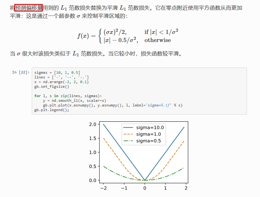
1、L1/L2(MSE)/Smooth L1 Loss
-
L1、L2 Loss(欧式损失): M S E ( y _ , y ) = 1 n ∑ i = 1 n ( y _ ( i ) − y ( i ) ) 2 MSE(y_{\_}, y)= \frac{1}{n} \sum_{i=1}^{n}(y_{\_}^{(i)}-y^{(i)})^{2} MSE(y_,y)=n1∑i=1n(y_(i)−y(i))2
-
Smooth L1 Loss:它对噪声(outliers)更鲁棒,论文中效果较好的参数为 σ = 1.0 \sigma = 1.0 σ=1.0
-
Smooth L1 Loss 比 L1 Loss 或 L2 loss 好的原因?
-
回归损失函数在 TF 中的实现
# smooth-l1-loss def bbox_ohem_smooth_L1_loss(bbox_pred, bbox_target, label): sigma = tf.constant(1.0) threshold = 1.0 / (sigma ** 2) zeros_index = tf.zeros_like(label, dtype=tf.float32) valid_inds = tf.where(label != zeros_index, tf.ones_like(label, dtype=tf.float32), zeros_index) abs_error = tf.abs(bbox_pred - bbox_target) loss_smaller = 0.5 * ((abs_error * sigma) ** 2) loss_larger = abs_error - 0.5 / (sigma ** 2) smooth_loss = tf.reduce_sum(tf.where(abs_error < threshold, loss_smaller, loss_larger), axis=1) keep_num = tf.cast(tf.reduce_sum(valid_inds) * num_keep_radio, dtype=tf.int32) smooth_loss = smooth_loss * valid_inds _, k_index = tf.nn.top_k(smooth_loss, k=keep_num) smooth_loss_picked = tf.gather(smooth_loss, k_index) return tf.reduce_mean(smooth_loss_picked) # L2 Loss # bbox_pred: batch*4 # bbox_target: batch*4 # label:batch # label=1 or label=-1 then do regression # 正样本和 part 样本做 bbox regression, # 所有样本都做了 inference,只是取正样本和 part 样本来做 bbox regression 而已 def bbox_ohem(bbox_pred, bbox_target, label): zeros_index = tf.zeros_like(label, dtype=tf.float32) ones_index = tf.ones_like(label, dtype=tf.float32) valid_inds = tf.where(tf.equal(tf.abs(label), 1), ones_index, zeros_index) # 384 # (batch,) square_error = tf.square(bbox_pred - bbox_target) # 384*4 square_error = tf.reduce_sum(square_error, axis=1) # 384,每一个样本的左上右下差值的平方加和 # keep_num scalar num_valid = tf.reduce_sum(valid_inds) # 取得正样本和 part 样本的数目 # keep_num = tf.cast(num_valid*num_keep_radio,dtype=tf.int32) keep_num = tf.cast(num_valid, dtype=tf.int32) # keep valid index square_error, set 0 to invalid sample(neg, landmark) square_error = square_error * valid_inds # 384,将 neg 和 landmark 的 error 项设置为 0 _, k_index = tf.nn.top_k(square_error, k=keep_num) # 有必要,但是仅仅是取得 error 不为 0 的项,并没有做 ohem square_error = tf.gather(square_error, k_index) # 直接用 _ 做最后的 reduce_mean 不就行了?这不是多此一举吗? return tf.reduce_mean(square_error) -
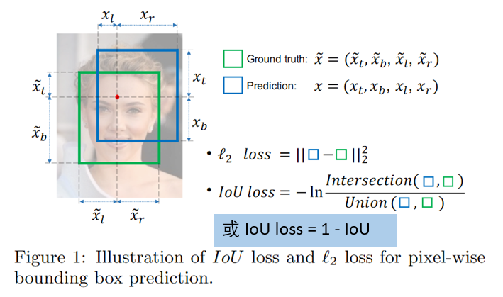
通过 4 个坐标点独立回归 Building boxes 的缺点:
- 检测
评价方式使用的是 IoU,而实际回归坐标框的时候是使用 4 个坐标点 - 通过4个点回归坐标框的方式是假设 4 个坐标点是相互独立的,没有考虑其
相关性,实际 4 个坐标点具有一定的相关性 - 基于 L1 和 L2 的距离的 loss 对于
尺度不具有不变性(大框较小框损失更大)
- 检测
2、IoU Loss
-
IoU loss 的优点:解决了 Smooth L1 系列变量
相互独立和不具有尺度不变性(大框较小框损失更大)的两大问题
-
IoU loss 的缺点:
- 预测框和真实框不相交时(IOU=0),不能反映出两个框的
距离的远近,此时损失函数不可导,IOU_Loss 无法优化 - 预测框和真实框相交时,无法反映
重合度大小,如下图所示,后面两个具有相同的 IOU,但是不能反映两个框是如何相交的
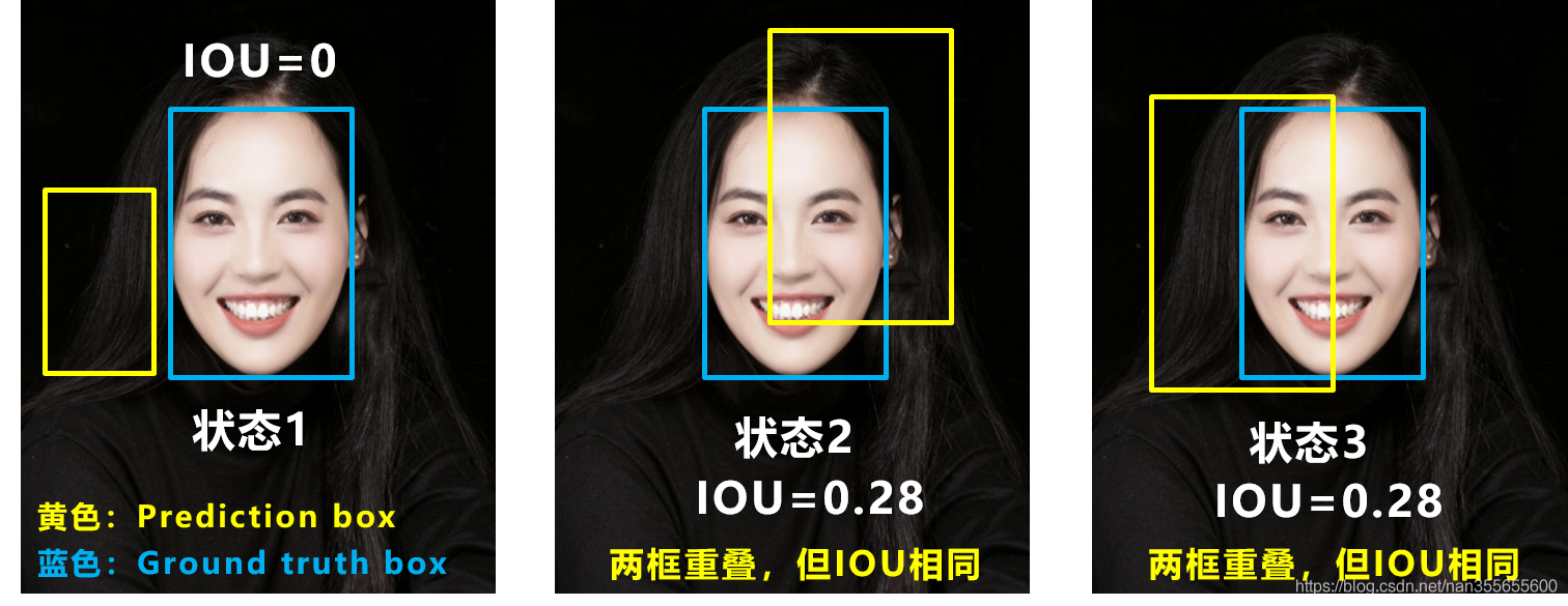
- 预测框和真实框不相交时(IOU=0),不能反映出两个框的
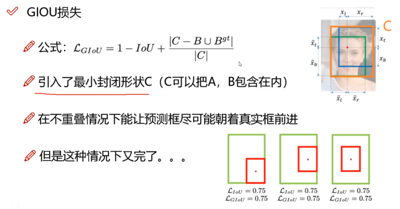
3、GIoU Loss
- GIoU Loss 的优点:在 IoU 的基础上引入了预测框和真实框的
最小外接矩形- 不仅关注重叠区域,还关注其他的非重叠区域,能更好的反映两者的重合度
- 当预测框和真实框不相交时,由于引入了预测框和真实框的最小外接矩形,最小化 GIoU Loss 会促使 Anchor 和 GT 框不断靠近
- GIoU Loss 的缺点:当两个框属于包含关系时,如下图所示,GIoU 会退化成 IoU,无法区分其相对位置关系(
无法反应中心点距离远近)
4、DIoU Loss(Distance-IoU Loss)
- DIoU 的优点:
- 能够直接最小化预测框和真实框的中心点距离加速收敛
- 还可以替换普通的 IoU 评价策略,应用于NMS 中,使得 NMS 得到的结果更加合理和有效
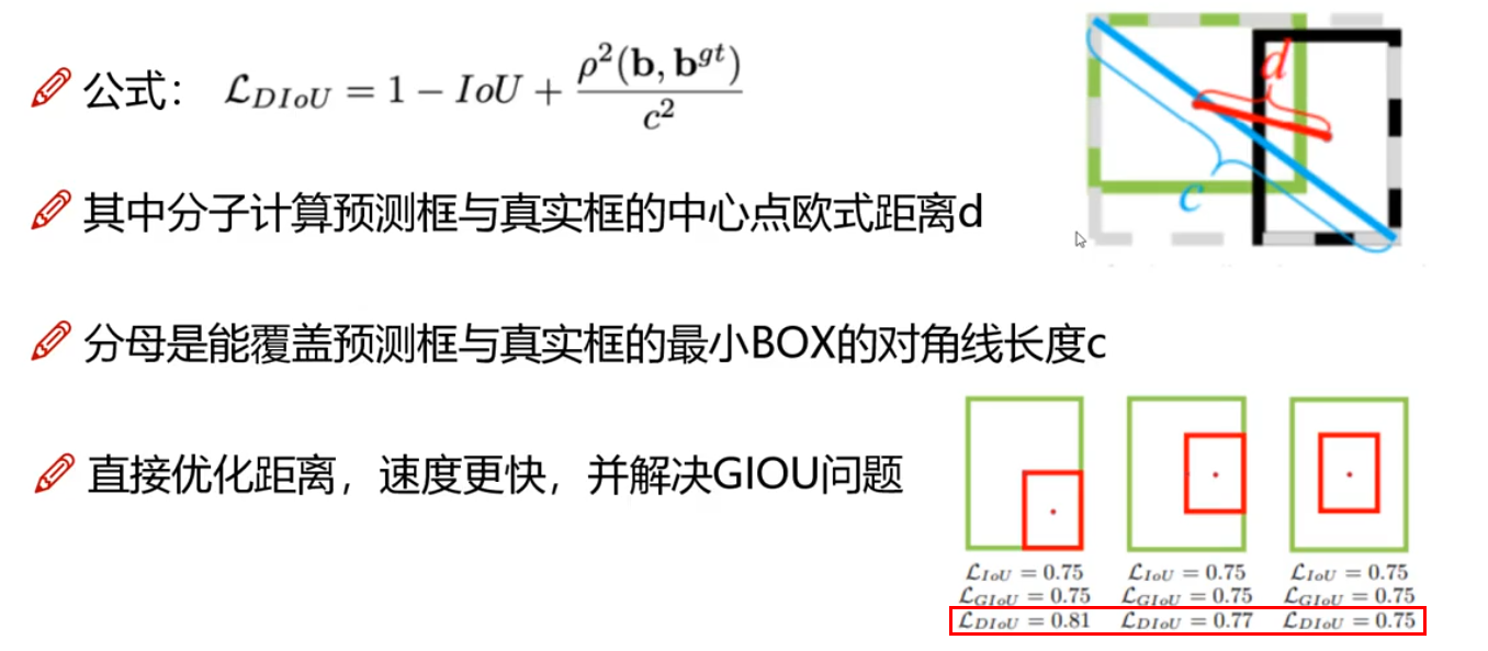
- DIoU 的缺点:未考虑 bbox 回归的长宽比
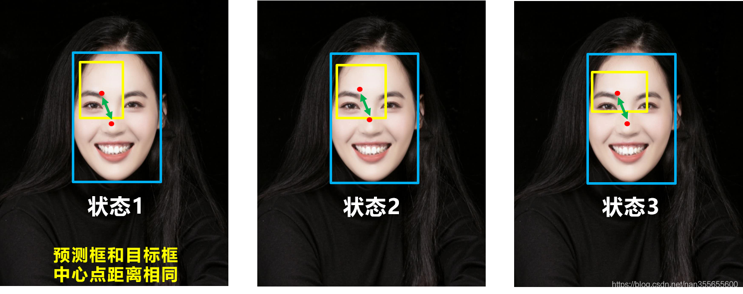
5、CIoU Loss(Complete-IoU Loss)
- CIoU 优缺点:在 DIoU 的基础上将 bbox 的长宽比考虑到损失函数中,进一步提升了回归精度
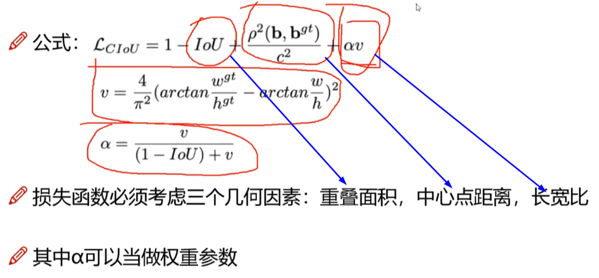
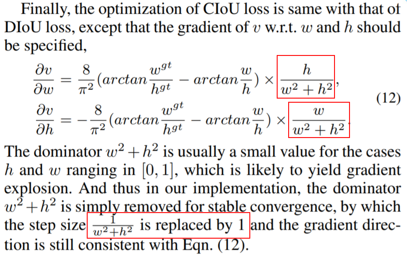
- 求导注意事项:
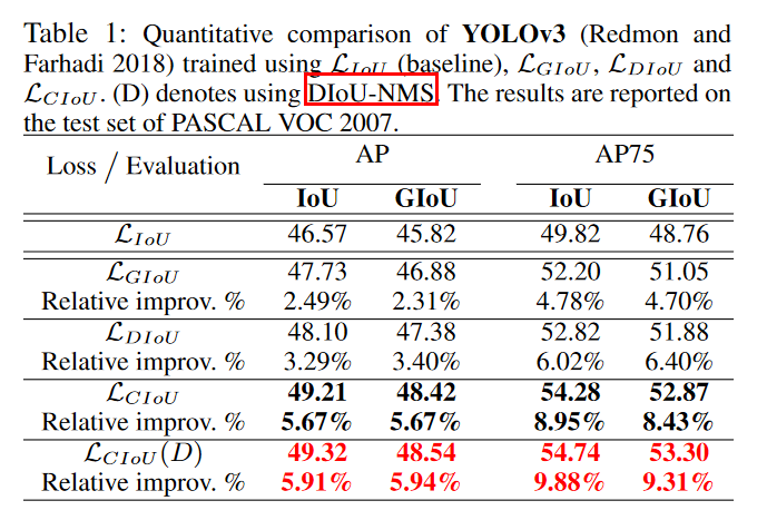
6、各种 IoU based loss 的效果及代码实现
def bbox_iou(box1, box2, x1y1x2y2=True, GIoU=False, DIoU=False, CIoU=False, eps=1e-7):
    # Returns the IoU of box1 to box2. box1 is 4, box2 is nx4
    box2 = box2.T

    # Get the coordinates of bounding boxes
    if x1y1x2y2:  # x1, y1, x2, y2 = box1
        b1_x1, b1_y1, b1_x2, b1_y2 = box1[0], box1[1], box1[2], box1[3]
        b2_x1, b2_y1, b2_x2, b2_y2 = box2[0], box2[1], box2[2], box2[3]
    else:  # transform from xywh to xyxy
        b1_x1, b1_x2 = box1[0] - box1[2] / 2, box1[0] + box1[2] / 2
        b1_y1, b1_y2 = box1[1] - box1[3] / 2, box1[1] + box1[3] / 2
        b2_x1, b2_x2 = box2[0] - box2[2] / 2, box2[0] + box2[2] / 2
        b2_y1, b2_y2 = box2[1] - box2[3] / 2, box2[1] + box2[3] / 2

    # Intersection area
    inter = (torch.min(b1_x2, b2_x2) - torch.max(b1_x1, b2_x1)).clamp(0) * \
            (torch.min(b1_y2, b2_y2) - torch.max(b1_y1, b2_y1)).clamp(0)

    # Union Area
    w1, h1 = b1_x2 - b1_x1, b1_y2 - b1_y1 + eps
    w2, h2 = b2_x2 - b2_x1, b2_y2 - b2_y1 + eps
    union = w1 * h1 + w2 * h2 - inter + eps

    iou = inter / union
    if GIoU or DIoU or CIoU:
    	# 计算闭包区域
        cw = torch.max(b1_x2, b2_x2) - torch.min(b1_x1, b2_x1)  # convex (smallest enclosing box) width
        ch = torch.max(b1_y2, b2_y2) - torch.min(b1_y1, b2_y1)  # convex height
        if CIoU or DIoU:  # Distance or Complete IoU https://arxiv.org/abs/1911.08287v1
            c2 = cw ** 2 + ch ** 2 + eps  # convex diagonal squared
            rho2 = ((b2_x1 + b2_x2 - b1_x1 - b1_x2) ** 2 +
                    (b2_y1 + b2_y2 - b1_y1 - b1_y2) ** 2) / 4  # center distance squared,计算中心点距离
            if DIoU:
                return iou - rho2 / c2  # DIoU
            elif CIoU:  # https://github.com/Zzh-tju/DIoU-SSD-pytorch/blob/master/utils/box/box_utils.py#L47
                v = (4 / math.pi ** 2) * torch.pow(torch.atan(w2 / h2) - torch.atan(w1 / h1), 2)
                with torch.no_grad():
                    alpha = v / (v - iou + (1 + eps))
                return iou - (rho2 / c2 + v * alpha)  # CIoU
        else:  # GIoU https://arxiv.org/pdf/1902.09630.pdf
            c_area = cw * ch + eps  # convex area
            return iou - (c_area - union) / c_area  # GIoU
    else:
        return iou  # IoU
三、SSD 中的损失函数
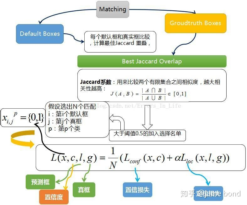
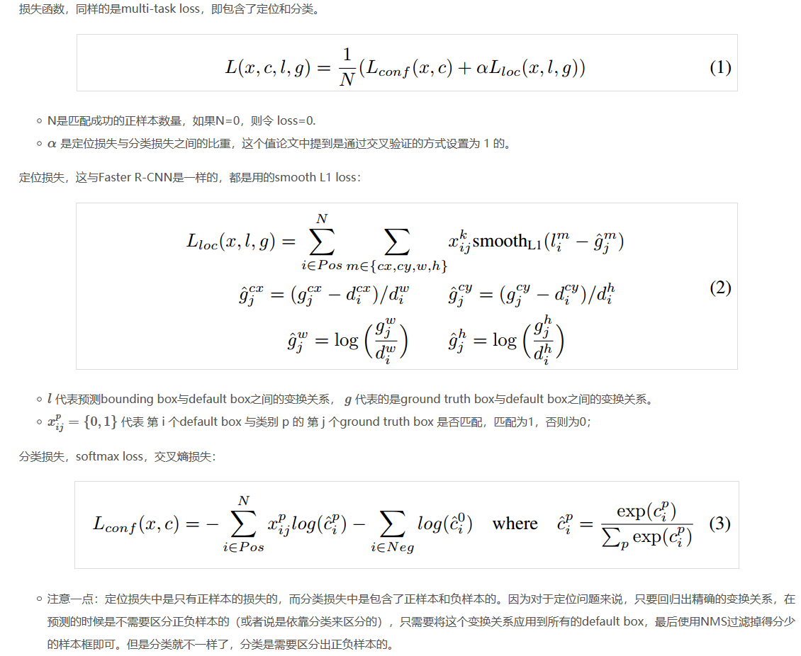
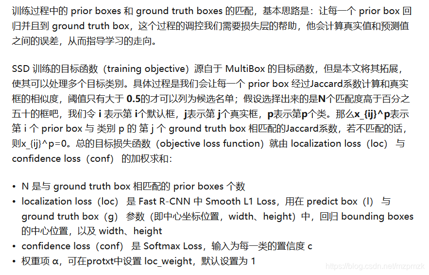
四、目标检测中回归的原理
1、为什么要做 bbox regression?
回归目的:提高目标定位的精度!
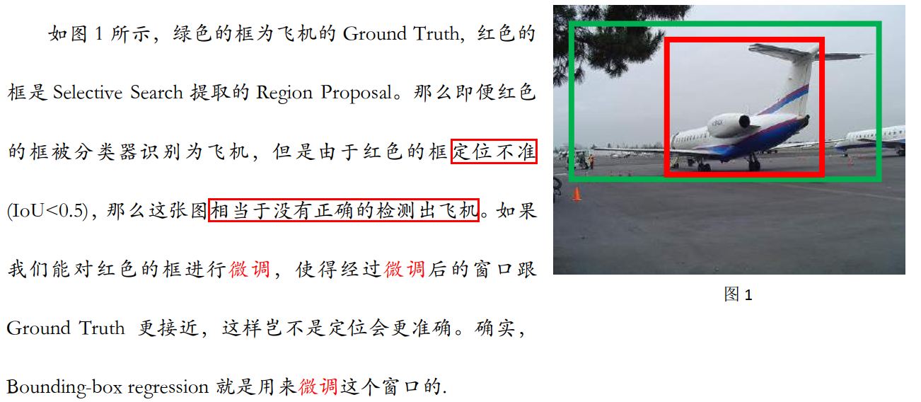
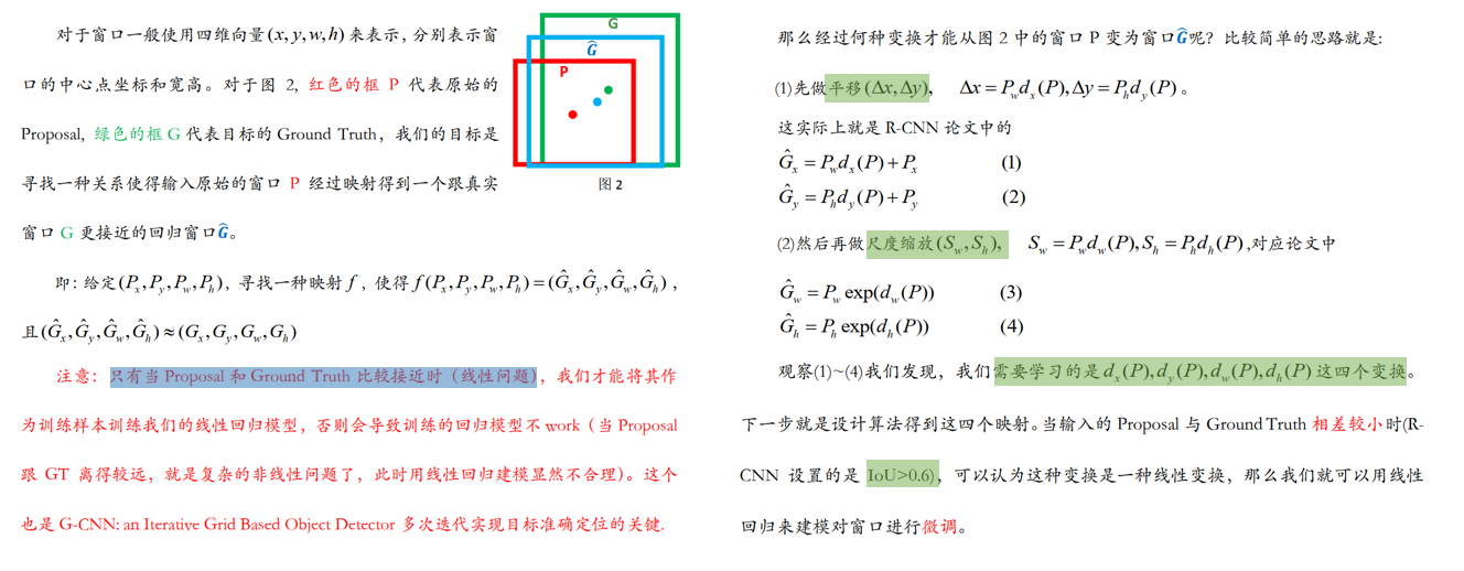
2、回归的对象是什么?
回归对象:相对 prior box(anchor box or propoal) 的平移和缩放量,这样可以使得模型有一个较好的搜索起点
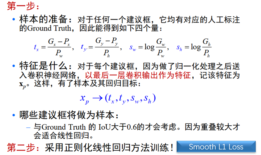
3、回归模型怎么训练?
- 训练方法:
- 对每一个 prior box(anchor box or propoal) 进行 labeling,只选取其中的正样本(eg: IoU>0.6)来做回归
- 计算 prior box 和其对应的 groud truth box 间的平移和缩放量
- 注意:这里的平移和缩放量
除以了prior box 的宽和高(宽和高变换到对数域)做归一化处理,因为图像中各个框的位置远近以及形状大小各异,这样做能使偏移量的分布更均匀从而更容易拟合
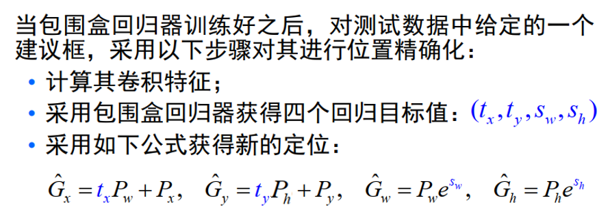
4、回归模型怎么测试?
输入:prior box 的坐标 ( P x , P y , P w , P h ) (P_x, P_y, P_w, P_h) (Px,Py,Pw,Ph),其实真正的输入是这个窗口对应的
CNN 特征
输出:prior box 经过模型回归后的坐标 ( t x , t y , s w , s h ) (t_x, t_y, s_w, s_h) (tx,ty,sw,sh),然后再做一下反归一化就可以得到其真实坐标
// 注意这里加了 prior_variance 参数(便于梯度更好的回传),一般为 [0.1, 0.1, 0.2, 0.2]
// variance is encoded in bbox, we need to scale the offset accordingly.
decode_bbox_center_x = prior_variance[0] * bbox.xmin() * prior_width + prior_center_x;
decode_bbox_center_y = prior_variance[1] * bbox.ymin() * prior_height + prior_center_y;
decode_bbox_width = exp(prior_variance[2] * bbox.xmax()) * prior_width;
decode_bbox_height = exp(prior_variance[3] * bbox.ymax()) * prior_height;

// 然后转成两个坐标的形式
decode_bbox->set_xmin(decode_bbox_center_x - decode_bbox_width / 2.);
decode_bbox->set_ymin(decode_bbox_center_y - decode_bbox_height / 2.);
decode_bbox->set_xmax(decode_bbox_center_x + decode_bbox_width / 2.);
decode_bbox->set_ymax(decode_bbox_center_y + decode_bbox_height / 2.);
五、参考资料
1、TensorFLow 中的损失函数
2、请问faster rcnn和ssd 中为什么用smooth l1 loss,和l2有什么区别?
3、L1&L2 正则化
4、bounding box regression detail(CaffeCN)
5、论文阅读: RetinaNet !!
6、何恺明大神的「Focal Loss」,如何更好地理解?
7、5分钟理解Focal Loss与GHM——解决样本不平衡利器 !!!
8、Imbalance Problems in Object Detection: A Review
9、详解各种iou损失函数的计算方式(iou、giou、ciou、diou)


 被折叠的 条评论
为什么被折叠?
被折叠的 条评论
为什么被折叠?
 到【灌水乐园】发言


