


一、导入库
import numpy as np
import torch
1.1 定义数组以及张量
array = [[1, 2, 3], [4, 5, 6]]
first_array = np.array(array)  # 2x3 array
print("Array Type: {}".format(type(first_array)))  # type
print("Array Shape: {}".format(np.shape(first_array)))  # shape
print(first_array)
tensor = torch.Tensor(array)
print("Array Type: {}".format(tensor.type))
print("Array Shape: {}".format(tensor.shape))
结果:
Array Type: <class 'numpy.ndarray'>
Array Shape: (2, 3)
[[1 2 3]
 [4 5 6]]
tensor([[1., 2., 3.],
        [4., 5., 6.]])
Array Type: <built-in method type of Tensor object at 0x000001E95BB8DF10>
Array Shape: torch.Size([2, 3])
需注意,张量中数据类型为浮点型
1.1.1 标量、向量、矩阵、张量
- 标量(Scalar):只有大小,没有方向,如1,2,3等等。
- 向量(Vector):有大小和方向,如向量(1,2,3)。
- 矩阵(Matrix):由几个向量合并而成,如[1,2;3,4] 。
- 张量(Tensor):张量可以是任意维度,零维时是标量,一维时为向量,二维时为矩阵,还有三维、四维、五维等等。
1.1.2 矩阵matrix和数组array的区别
- matrix只能是2维的,而array可以是任意维数
import numpy as np a = np.random.rand(2, 2, 2) print(a) #结果:[[[0.38070197 0.82117218] [0.33945994 0.64425157]] [[0.60596089 0.17094728] [0.94860822 0.06847263]]] b = np.mat(np.random.rand(2, 2, 2)) #结果:ValueError("shape too large to be a matrix.") - 运算规则不同
#数组运算:
数与数组加减:k+/-A        %k加或减A的每个元素
数组乘数组:  A.*B         %对应元素相乘
数组乘方:  A.^k         %A的每个元素k次方;k.^A,分别以k为底A的各元素为指数求幂值
数除以数组:  k./A和A./k   %k分别被A的元素除
数组除法:    左除A.\B右除B./A,对应元素相除

#矩阵运算:
数与矩阵加减:k+/-A             %等价于k*ones(size(A))+/-A
矩阵乘法:    A*B               %按数学定义的矩阵乘法规则
矩阵乘方:  A^k               %k个矩阵A相乘
矩阵除法:    左除A\B右除B/A    %分别为AX=B和XA=B的解
1.1.3 数组array与张量tensor的区别
任意数组都可以被视为张量,而张量不能都被视为数组。因为张量具有任意维度(从0维到任意维),而数组只有一维到多维。并且数组只包含相同类型的数据,而张量包含不同类型的数据。张量是神经网络计算的基本单元,tensor可以轻易地进行卷积、激活、上下采样和微分求导等操作,而numpy数组则不行,因此需要将数组转化为张量进行处理。区别于numpy数组,tensor类型可以在GPU上进行加速计算。
1.2 数组和张量相互转化
# random numpy array
array = np.random.rand(2, 2)
print("{} {}\n".format(type(array), array))
# from numpy to tensor
from_numpy_to_tensor = torch.from_numpy(array)
print("{}\n".format(from_numpy_to_tensor))
# from tensor to numpy
tensor = from_numpy_to_tensor
from_tensor_to_numpy = tensor.numpy()
print("{} {}\n".format(type(from_tensor_to_numpy), from_tensor_to_numpy))
结果:
<class 'numpy.ndarray'> [[0.56216701 0.11552156]
 [0.37062749 0.11044086]]

tensor([[0.5622, 0.1155],
        [0.3706, 0.1104]], dtype=torch.float64)

<class 'numpy.ndarray'> [[0.56216701 0.11552156]
 [0.37062749 0.11044086]]
1.3 张量运算
# create tensor
tensor = torch.ones(4, 4)
print("\n", tensor)

# Resize
print("{}{}\n".format(tensor.view(8,2).shape, tensor.view(8,2)))

# Addition +
print("Addition: {}\n".format(torch.add(tensor, tensor)))

# Subtraction -
print("Subtraction: {}\n".format(tensor.sub(tensor)))

# Element wise multiplication *
print("Element wise multiplication: {}\n".format(torch.mul(tensor, tensor)))

# Element wise division /
print("Element wise division: {}\n".format(torch.div(tensor, tensor)))

# Mean
tensor = torch.Tensor([1, 2, 3, 4, 5])
print("Mean: {}".format(tensor.mean()))

# Standart deviation (std) 标准差
print("std: {}".format(tensor.std()))
结果:
 tensor([[1., 1., 1., 1.],
        [1., 1., 1., 1.],
        [1., 1., 1., 1.],
        [1., 1., 1., 1.]])
torch.Size([8, 2])tensor([[1., 1.],
        [1., 1.],
        [1., 1.],
        [1., 1.],
        [1., 1.],
        [1., 1.],
        [1., 1.],
        [1., 1.]])

Addition: tensor([[2., 2., 2., 2.],
        [2., 2., 2., 2.],
        [2., 2., 2., 2.],
        [2., 2., 2., 2.]])

Subtraction: tensor([[0., 0., 0., 0.],
        [0., 0., 0., 0.],
        [0., 0., 0., 0.],
        [0., 0., 0., 0.]])

Element wise multiplication: tensor([[1., 1., 1., 1.],
        [1., 1., 1., 1.],
        [1., 1., 1., 1.],
        [1., 1., 1., 1.]])

Element wise division: tensor([[1., 1., 1., 1.],
        [1., 1., 1., 1.],
        [1., 1., 1., 1.],
        [1., 1., 1., 1.]])

Mean: 3.0
std: 1.5811388492584229
二、autograd自动微分
import torch
from torch.autograd import Variable
x = Variable(torch.ones(2), requires_grad = True)
print(x)
y = 4 * x ** 2
print(y)
y_1 = y.norm() #2范数
print(y_1)
y_1.backward()
print(x.grad)
结果:
tensor([1., 1.], requires_grad=True)
tensor([4., 4.], grad_fn=<MulBackward0>)
tensor(5.6569, grad_fn=<LinalgVectorNormBackward0>)
tensor([5.6569, 5.6569])
三、线性回归
import numpy as np # 线性代数操作
# import pandas as pd # 数据处理,CSV文件读取等,这里没用到所以注释
# As a car company we collect this data from previous selling
# lets define car prices
# import variable from pytorch library
from torch.autograd import Variable # 从 PyTorch 库中导入 Variable 类
import torch
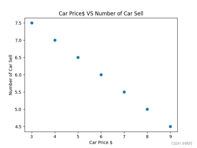
car_prices_array = [3, 4, 5, 6, 7, 8, 9]
car_price_np = np.array(car_prices_array, dtype=np.float32)
car_price_np = car_price_np.reshape(-1, 1)
car_price_tensor = Variable(torch.from_numpy(car_price_np))
# lets define number of car sell
number_of_car_sell_array = [7.5, 7, 6.5, 6.0, 5.5, 5.0, 4.5]
number_of_car_sell_np = np.array(number_of_car_sell_array, dtype=np.float32)
number_of_car_sell_np = number_of_car_sell_np.reshape(-1, 1)
number_of_car_sell_tensor = Variable(torch.from_numpy(number_of_car_sell_np))
# lets visualize our data
import matplotlib.pyplot as plt
plt.scatter(car_prices_array,number_of_car_sell_array)
plt.xlabel("Car Price $")
plt.ylabel("Number of Car Sell")
plt.title("Car Price$ VS Number of Car Sell")
plt.show()
# Linear Regression with Pytorch
# libraries
import torch
from torch.autograd import Variable
import torch.nn as nn
import warnings
warnings.filterwarnings("ignore")
# create class
class LinearRegression(nn.Module):
def __init__(self, input_size, output_size):
# super function. It inherits from nn.Module and we can access everythink in nn.Module
super(LinearRegression, self).__init__()
# Linear function.
self.linear = nn.Linear(input_dim, output_dim)
def forward(self, x):
return self.linear(x)
# define model
input_dim = 1
output_dim = 1
model = LinearRegression(input_dim, output_dim) # input and output size are 1
# MSE
mse = nn.MSELoss()
# Optimization (find parameters that minimize error)
learning_rate = 0.02 # how fast we reach best parameters
optimizer = torch.optim.SGD(model.parameters(), lr=learning_rate)
# train model
loss_list = []
iteration_number = 1001
for iteration in range(iteration_number):
# optimization
optimizer.zero_grad()
# Forward to get output
results = model(car_price_tensor)
# Calculate Loss
loss = mse(results, number_of_car_sell_tensor)
# backward propagation
loss.backward()
# Updating parameters
optimizer.step()
# store loss
loss_list.append(loss.data)
# print loss
if (iteration % 50 == 0):
print('epoch {}, loss {}'.format(iteration, loss.data))
plt.plot(range(iteration_number), loss_list)
plt.xlabel("Number of Iterations")
plt.ylabel("Loss")
plt.show()
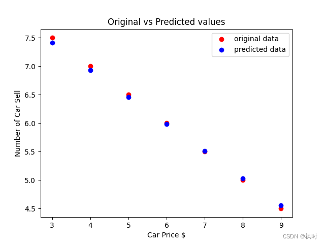
# predict our car price
predicted = model(car_price_tensor).data.numpy()
plt.scatter(car_prices_array, number_of_car_sell_array, label="original data", color="red")
plt.scatter(car_prices_array, predicted, label="predicted data", color="blue")
# predict if car price is 10$, what will be the number of car sell
# predicted_10 = model(torch.from_numpy(np.array([10]))).data.numpy()
# plt.scatter(10,predicted_10.data,label = "car price 10$",color ="green")
plt.legend()
plt.xlabel("Car Price $")
plt.ylabel("Number of Car Sell")
plt.title("Original vs Predicted values")
plt.show()3.1 结果
epoch 0, loss 21.220523834228516
epoch 50, loss 4.4300127029418945
epoch 100, loss 2.9935452938079834
epoch 150, loss 2.0228641033172607
epoch 200, loss 1.3669337034225464
epoch 250, loss 0.9236940145492554
epoch 300, loss 0.6241793632507324
epoch 350, loss 0.4217838943004608
epoch 400, loss 0.28501737117767334
epoch 450, loss 0.19259829819202423
epoch 500, loss 0.13014636933803558
epoch 550, loss 0.08794522285461426
epoch 600, loss 0.05942844599485397
epoch 650, loss 0.040158454328775406
epoch 700, loss 0.027136819437146187
epoch 750, loss 0.018337488174438477
epoch 800, loss 0.012391497381031513
epoch 850, loss 0.008373329415917397
epoch 900, loss 0.005658137612044811
epoch 950, loss 0.0038234065286815166
epoch 1000, loss 0.002583693014457822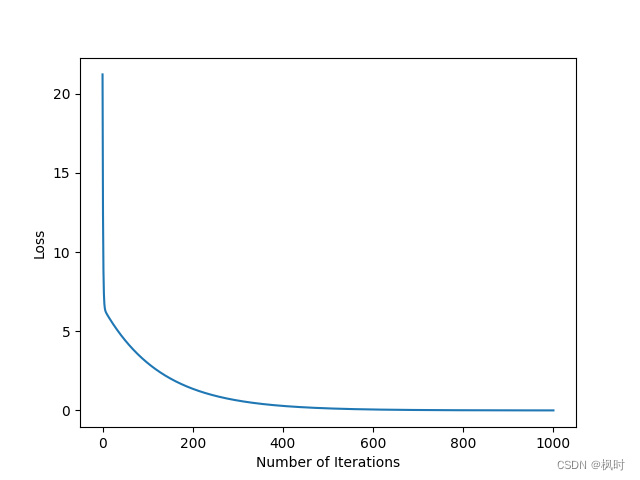
3.2 补充:reshape函数
numpy.reshape()函数用于改变数组的形状。
函数参数:reshape(a, newshape, order)
import numpy as np
x = np.array([[1,2,3], [4,5,6]])

np.reshape(x, (3, 2))
#输出:[[1 2 3]
             [4 5 6]]

x = np.reshape(x, 6) #整数默认变为一维数组,默认为行
#输出:[1 2 3 4 5 6]

x = np.reshape(x, (-1, 2)) #负数为模糊控制,由另一个元素控制,这里固定2列
#输出:[[1 2]
        [3 4]
        [5 6]]

x = np.reshape(x, (2, -1))
#输出:[[1 2 3]
        [4 5 6]]

x = np.reshape(x, (-1, 2), order='f')  # f为优先按列排序,这里即按列数分两行, 默认为行,即order = c
输出:[[1 5]
       [4 3]
       [2 6]]
3.3 关于Variable
Variable用于包装张量并提供自动微分功能,但现在的Pytorch张量本身具有自动微分功能,因此不需要额外的包装。
参考:https://www.cnblogs.com/zhuozige/p/14691225.html
https://www.kaggle.com/code/kanncaa1/pytorch-tutorial-for-deep-learning-lovers/notebook


 196
196

 被折叠的 条评论
为什么被折叠?
被折叠的 条评论
为什么被折叠?
 到【灌水乐园】发言


