d2l过拟合章节引申出多项式回归流程

在第四章节过拟合例子中，其中构造的多项式回归操作流程吸引笔者兴趣，为提升代码能力故做此博文，详细debug该操作。

核心任务：上一个softmax数据集是图片，这里数据集是随机生成数字，且利用自创多项式进行拟合！

目录

1.生成多项式

2.定义损失计算函数

3.训练函数（改正显示数值版本）

4.最终训练命令行

---

1.生成多项式

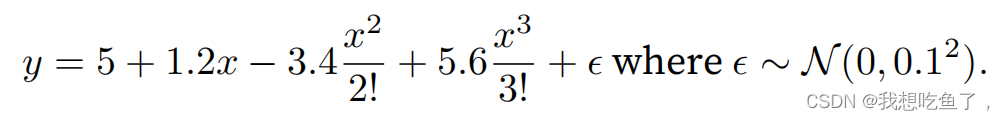
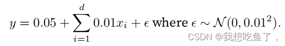
目标，生成如下多项式所运算的标签值数据集

具体流程代码：

max_degree = 20 # 多项式的最⼤阶数
n_train, n_test = 100, 100 # 训练和测试数据集⼤⼩
true_w = np.zeros(max_degree) # 分配⼤量的空间
true_w[0:4] = np.array([5, 1.2, -3.4, 5.6]) # 其他的全是0

features = np.random.normal(size=(n_train + n_test, 1))
np.random.shuffle(features)
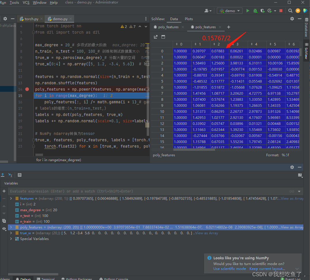
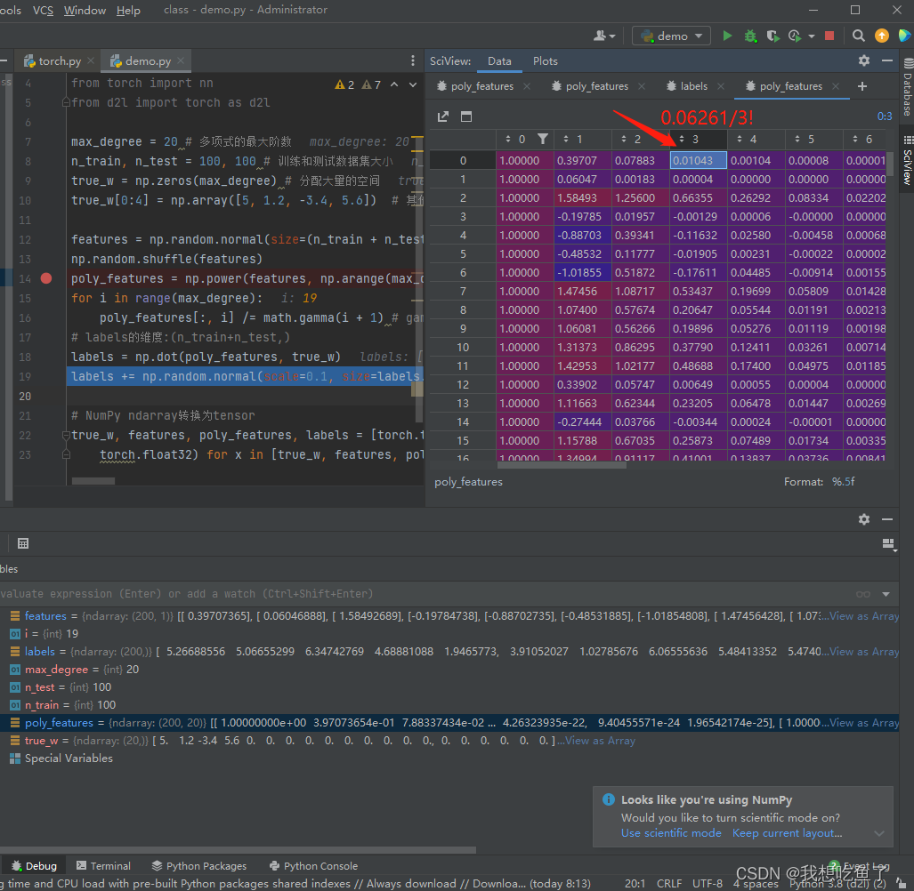
poly_features = np.power(features, np.arange(max_degree).reshape(1, -1))
for i in range(max_degree):
    poly_features[:, i] /= math.gamma(i + 1) # gamma(n)=(n-1)!
# labels的维度:(n_train+n_test,)
labels = np.dot(poly_features, true_w)
labels += np.random.normal(scale=0.1, size=labels.shape)

这里为了对比，首先设置max_degree=20，在后续对比中可以取到x20次方多项式。

np.random.normal表示随机生成满足正态分布的数张量,生成了(200,1)个x点。

np.power(a,b)为计算a的b次方，例子如下所示：最后输出的是shape是(2,3),所以对一个(2,1)的张量进行一个(1,3)的power操作，讲(2,1)中的每个元素分别进行(1,3)中的指数操作，最终生成(2,3)的结果，其中1，3表示在原先的1元素对应3元素的指数次方操作。

g = np.random.normal(size=(2, 1)) 
n = np.arange(3).reshape(1,-1)
np.power(g,n), n, g

'''
(array([[ 1.        ,  0.08497032,  0.00721995],
        [ 1.        , -0.76966152,  0.59237886]]),
 array([[0, 1, 2]]),
 array([[ 0.08497032],
        [-0.76966152]]))
'''

回到这个例子中，经过power操作后，将原先的features(200,1)的xi元素进行了上述指数操作，生成的poly_features为（200，20）的向量，每一列表示对应元素对应次方，例如0，3表示features中0位置(第一个)数的3次方，即对应多项式中的x3次方！

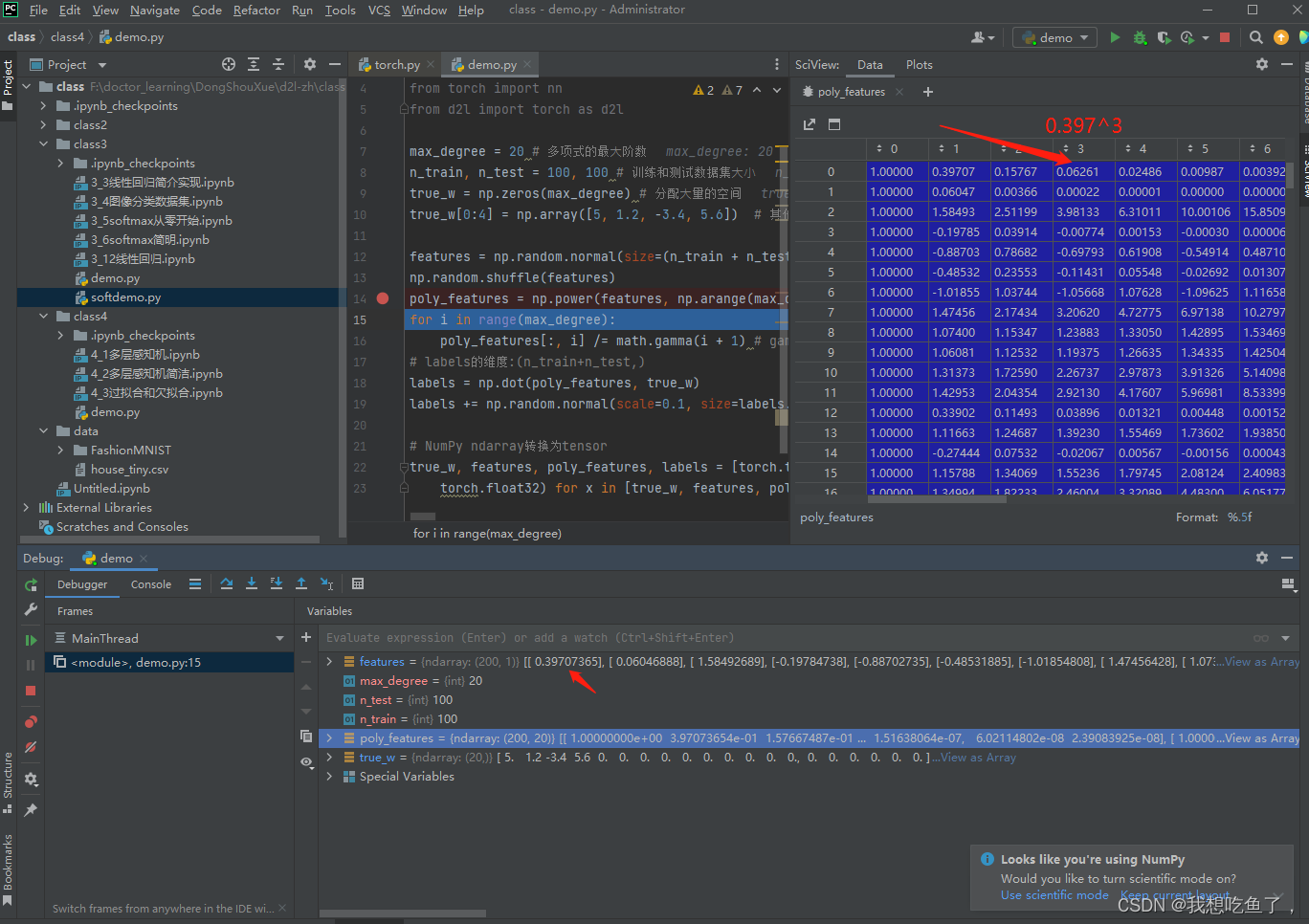
 下一个for循环表示在多项式函数中的对指数除对应分母，如下两图所示：将poly_featrues如第一个数x的0次方，除0！，即为1，第二个数即x的1次方，除1！，即为x本身，第三个数x的2次方，除2！即为图中所示...

最终得到的是poly_features=(x^o,x,x^2/2!,x^3/3!...,x^20/20!)

 接下来进行np.dot操作，表示两个向量的内积，即(200,20)与(20)的内积 ,得到的是每一行(x^o/0!,x/1!,x^2/2!,x^3/3!...,x^20/20!)与true_w内积加和，再通过添加随机噪声，最终生成y的多项式表达式，这里相当于随机带入了满足正态分布0，1的两百个x值得到的满足上述任务多项式的200个y标签值。

再进行格式转换，将numpy转为tensor方便后续操作:

# NumPy ndarray转换为tensor
true_w, features, poly_features, labels = [torch.tensor(x, dtype=
    torch.float32) for x in [true_w, features, poly_features, labels]]

观察一下输出结果：其中[:2]表示从头读取到第2行，与[0:2]等价,表示输出前两个poly_features，每一行都是(x^o/0!,x/1!,x^2/2!,x^3/3!...,x^20/20!)

features.shape, features[:2], poly_features[:2, :], labels[:2], labels.shape

'''
(torch.Size([200, 1]),
 tensor([[0.1062],
         [0.2925]]),
 tensor([[1.0000e+00, 1.0621e-01, 5.6401e-03, 1.9967e-04, 5.3017e-06, 1.1262e-07,
          1.9935e-09, 3.0246e-11, 4.0155e-13, 4.7386e-15, 5.0328e-17, 4.8593e-19,
          4.3008e-21, 3.5137e-23, 2.6656e-25, 1.8874e-27, 1.2528e-29, 7.8271e-32,
          4.6183e-34, 2.5816e-36],
         [1.0000e+00, 2.9249e-01, 4.2774e-02, 4.1703e-03, 3.0494e-04, 1.7838e-05,
          8.6957e-07, 3.6334e-08, 1.3284e-09, 4.3171e-11, 1.2627e-12, 3.3575e-14,
          8.1835e-16, 1.8412e-17, 3.8466e-19, 7.5006e-21, 1.3711e-22, 2.3591e-24,
          3.8333e-26, 5.9010e-28]]),
 tensor([5.2388, 5.1748]),
 torch.Size([200]))
'''

2.定义损失计算函数

这里输入模型，数据集loader，损失函数，得到损失函数的平均值（总损失/样本总个数）

def evaluate_loss(net, data_iter, loss): #@save
    """评估给定数据集上模型的损失"""
    metric = d2l.Accumulator(2) # 损失的总和,样本数量
    for X, y in data_iter:
        out = net(X)
        y = y.reshape(out.shape)
        l = loss(out, y)
        metric.add(l.sum(), l.numel())
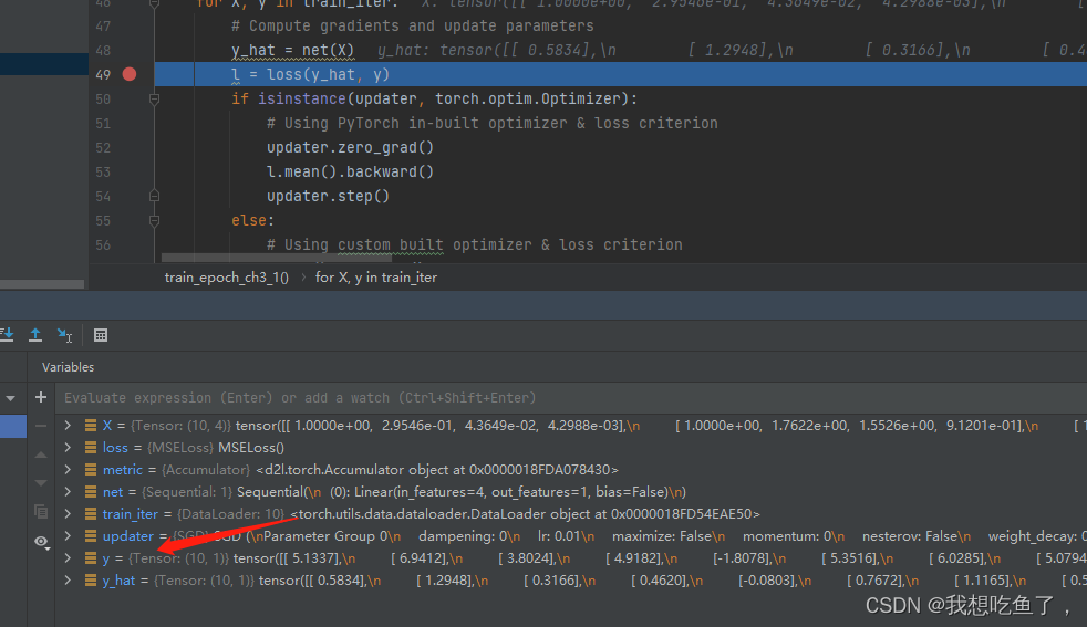
    return metric[0] / metric[1]

3.训练函数（改正显示数值版本）

这里面的mse即为1/2(y-y_hat)^2,net为很基础的全连接单层网络。

def train(train_features, test_features, train_labels, test_labels,
        num_epochs=400):
    loss = nn.MSELoss(reduction='none')
    input_shape = train_features.shape[-1]
    # 不设置偏置，因为我们已经在多项式中实现了它
    net = nn.Sequential(nn.Linear(input_shape, 1, bias=False))
    batch_size = min(10, train_labels.shape[0])
    train_iter = d2l.load_array((train_features, train_labels.reshape(-1,1)),
                                batch_size)
    test_iter = d2l.load_array((test_features, test_labels.reshape(-1,1)),
                                batch_size, is_train=False)
    trainer = torch.optim.SGD(net.parameters(), lr=0.01)

    for epoch in range(num_epochs):
        train_metrics = d2l.train_epoch_ch3(net, train_iter, loss, trainer)
        if epoch == 0 or (epoch + 1) % 20 == 0:
            print(f'训练损失{train_metrics[0]:.5f},测试损失{evaluate_loss(net, test_iter, loss):.5f}')

 这里补充下load_array函数：输入x，y两个参数，x为自变量数值，在本模型中即为除了要训练的系数之外的所有值（以下面去4各维度为例，即为poly_features的前四列），y对应的是上述目标多项式计算的labels值。

def load_array(data_arrays, batch_size, is_train=True):
    """Construct a PyTorch data iterator.

    Defined in :numref:`sec_linear_concise`"""
    dataset = data.TensorDataset(*data_arrays)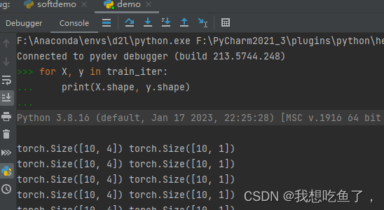
    return data.DataLoader(dataset, batch_size, shuffle=is_train)

该函数返回的是loader格式，即(bs,单个x维度),(bs,单个y维度)如下图所示：注意这个格式，y为(bs,单个y维度),这是因为在传入load_array的时候将labels进行了reshape(-1,1)操作，其原因在于这里使用的MSE损失函数，不是交叉熵！最后得到的y_hat都是二维的。

4.最终训练命令行

这是从多项式特征中选取前4个维度，即x^o/0!,x/1!,x^2/2!,x^3/3!。这里面前100行维训练，后100行为测试，取的维度越小模型越欠拟合，越大则越过拟合！

train(poly_features[:n_train, :4], poly_features[n_train:, :4],
      labels[:n_train], labels[n_train:])

5.多项式练习

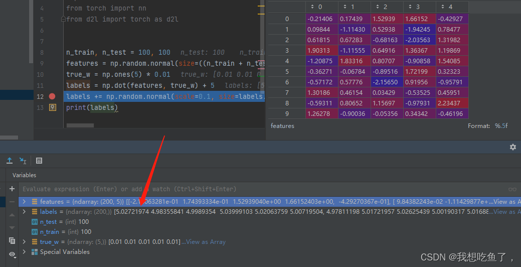
  下面式子，且噪声改为0.1，常数项改为5，d取5：

n_train, n_test = 100, 100
features = np.random.normal(size=((n_train + n_test), 5))
true_w = np.ones(5) * 0.01
labels = np.dot(features, true_w) + 5
labels += np.random.normal(scale=0.1, size=labels.shape)
print(labels)

 注意，在使用np.dot计算内积的时候，要保持第一参数的列数等于第二参数的向量元素数。

 结果：符合该多项式要求