第二周2--具有神经网络思维的Logistic回归（编程）

```python
# -*- coding: utf-8 -*-
"""
"""

import numpy as np
import matplotlib.pyplot as plt
import h5py
from lr_utils import load_dataset

train_set_x_orig , train_set_y , test_set_x_orig , test_set_y , classes = load_dataset()

m_train = train_set_y.shape[1] #训练集里图片的数量。
m_test = test_set_y.shape[1] #测试集里图片的数量。
num_px = train_set_x_orig.shape[1] #训练、测试集里面的图片的宽度和高度（均为64x64）。

#现在看一看我们加载的东西的具体情况
print ("训练集的数量: m_train = " + str(m_train))
print ("测试集的数量 : m_test = " + str(m_test))
print ("每张图片的宽/高 : num_px = " + str(num_px))
print ("每张图片的大小 : (" + str(num_px) + ", " + str(num_px) + ", 3)")
print ("训练集_图片的维数 : " + str(train_set_x_orig.shape))
print ("训练集_标签的维数 : " + str(train_set_y.shape))
print ("测试集_图片的维数: " + str(test_set_x_orig.shape))
print ("测试集_标签的维数: " + str(test_set_y.shape))

#将训练集的维度降低并转置。
train_set_x_flatten  = train_set_x_orig.reshape(train_set_x_orig.shape[0],-1).T
#将测试集的维度降低并转置。
test_set_x_flatten = test_set_x_orig.reshape(test_set_x_orig.shape[0], -1).T

print ("训练集降维最后的维度： " + str(train_set_x_flatten.shape))
print ("训练集_标签的维数 : " + str(train_set_y.shape))
print ("测试集降维之后的维度: " + str(test_set_x_flatten.shape))
print ("测试集_标签的维数 : " + str(test_set_y.shape))

train_set_x = train_set_x_flatten / 255
test_set_x = test_set_x_flatten / 255

def sigmoid(z):
    """
    参数：
        z  - 任何大小的标量或numpy数组。

    返回：
        s  -  sigmoid（z）
    """
    s = 1 / (1 + np.exp(-z))
    return s

def initialize_with_zeros(dim):
    """
        此函数为w创建一个维度为（dim，1）的0向量，并将b初始化为0。

        参数：
            dim  - 我们想要的w矢量的大小（或者这种情况下的参数数量）

        返回：
            w  - 维度为（dim，1）的初始化向量。
            b  - 初始化的标量（对应于偏差）
    """
    w = np.zeros(shape = (dim,1))
    b = 0
    #使用断言来确保我要的数据是正确的
    assert(w.shape == (dim, 1)) #w的维度是(dim,1)
    assert(isinstance(b, float) or isinstance(b, int)) #b的类型是float或者是int

    return (w , b)

def propagate(w, b, X, Y):
    """
    实现前向和后向传播的成本函数及其梯度。
    参数：
        w  - 权重，大小不等的数组（num_px * num_px * 3，1）
        b  - 偏差，一个标量
        X  - 矩阵类型为（num_px * num_px * 3，训练数量）
        Y  - 真正的“标签”矢量（如果非猫则为0，如果是猫则为1），矩阵维度为(1,训练数据数量)

    返回：
        cost- 逻辑回归的负对数似然成本
        dw  - 相对于w的损失梯度，因此与w相同的形状
        db  - 相对于b的损失梯度，因此与b的形状相同
    """
    m = X.shape[1]

    #正向传播
    A = sigmoid(np.dot(w.T,X) + b) #计算激活值，请参考公式2。
    cost = (- 1 / m) * np.sum(Y * np.log(A) + (1 - Y) * (np.log(1 - A))) #计算成本，请参考公式3和4。

    #反向传播
    dw = (1 / m) * np.dot(X, (A - Y).T) #请参考视频中的偏导公式。
    db = (1 / m) * np.sum(A - Y) #请参考视频中的偏导公式。

    #使用断言确保我的数据是正确的
    assert(dw.shape == w.shape)
    assert(db.dtype == float)
    cost = np.squeeze(cost)
    assert(cost.shape == ())

    #创建一个字典，把dw和db保存起来。
    grads = {
                "dw": dw,
                "db": db
             }
    return (grads , cost)

def optimize(w , b , X , Y , num_iterations , learning_rate , print_cost = False):
    """
    此函数通过运行梯度下降算法来优化w和b

    参数：
        w  - 权重，大小不等的数组（num_px * num_px * 3，1）
        b  - 偏差，一个标量
        X  - 维度为（num_px * num_px * 3，训练数据的数量）的数组。
        Y  - 真正的“标签”矢量（如果非猫则为0，如果是猫则为1），矩阵维度为(1,训练数据的数量)
        num_iterations  - 优化循环的迭代次数
        learning_rate  - 梯度下降更新规则的学习率
        print_cost  - 每100步打印一次损失值

    返回：
        params  - 包含权重w和偏差b的字典
        grads  - 包含权重和偏差相对于成本函数的梯度的字典
        成本 - 优化期间计算的所有成本列表，将用于绘制学习曲线。

    提示：
    我们需要写下两个步骤并遍历它们：
        1）计算当前参数的成本和梯度，使用propagate（）。
        2）使用w和b的梯度下降法则更新参数。
    """

    costs = []

    for i in range(num_iterations):

        grads, cost = propagate(w, b, X, Y)

        dw = grads["dw"]
        db = grads["db"]

        w = w - learning_rate * dw
        b = b - learning_rate * db

        #记录成本
        if i % 100 == 0:
            costs.append(cost)
        #打印成本数据
        if (print_cost) and (i % 100 == 0):
            print("迭代的次数: %i ， 误差值： %f" % (i,cost))

    params  = {
                "w" : w,
                "b" : b }
    grads = {
            "dw": dw,
            "db": db } 
    return (params , grads , costs)

def predict(w , b , X ):
    """
    使用学习逻辑回归参数logistic （w，b）预测标签是0还是1，

    参数：
        w  - 权重，大小不等的数组（num_px * num_px * 3，1）
        b  - 偏差，一个标量
        X  - 维度为（num_px * num_px * 3，训练数据的数量）的数据

    返回：
        Y_prediction  - 包含X中所有图片的所有预测【0 | 1】的一个numpy数组（向量）

    """

    m  = X.shape[1] #图片的数量
    Y_prediction = np.zeros((1,m)) 
    w = w.reshape(X.shape[0],1)

    #计预测猫在图片中出现的概率
    A = sigmoid(np.dot(w.T , X) + b)
    for i in range(A.shape[1]):
        #将概率a [0，i]转换为实际预测p [0，i]
        Y_prediction[0,i] = 1 if A[0,i] > 0.5 else 0
    #使用断言
    assert(Y_prediction.shape == (1,m))

    return Y_prediction

def model(X_train , Y_train , X_test , Y_test , num_iterations = 2000 , learning_rate = 0.5 , print_cost = False):
    """
    通过调用之前实现的函数来构建逻辑回归模型

    参数：
        X_train  - numpy的数组,维度为（num_px * num_px * 3，m_train）的训练集
        Y_train  - numpy的数组,维度为（1，m_train）（矢量）的训练标签集
        X_test   - numpy的数组,维度为（num_px * num_px * 3，m_test）的测试集
        Y_test   - numpy的数组,维度为（1，m_test）的（向量）的测试标签集
        num_iterations  - 表示用于优化参数的迭代次数的超参数
        learning_rate  - 表示optimize（）更新规则中使用的学习速率的超参数
        print_cost  - 设置为true以每100次迭代打印成本

    返回：
        d  - 包含有关模型信息的字典。
    """
    w , b = initialize_with_zeros(X_train.shape[0])

    parameters , grads , costs = optimize(w , b , X_train , Y_train,num_iterations , learning_rate , print_cost)

    #从字典“参数”中检索参数w和b
    w , b = parameters["w"] , parameters["b"]

    #预测测试/训练集的例子
    Y_prediction_test = predict(w , b, X_test)
    Y_prediction_train = predict(w , b, X_train)

    #打印训练后的准确性
    print("训练集准确性："  , format(100 - np.mean(np.abs(Y_prediction_train - Y_train)) * 100) ,"%")
    print("测试集准确性："  , format(100 - np.mean(np.abs(Y_prediction_test - Y_test)) * 100) ,"%")

    d = {
            "costs" : costs,
            "Y_prediction_test" : Y_prediction_test,
            "Y_prediciton_train" : Y_prediction_train,
            "w" : w,
            "b" : b,
            "learning_rate" : learning_rate,
            "num_iterations" : num_iterations }
    return d

d = model(train_set_x, train_set_y, test_set_x, test_set_y, num_iterations = 2000, learning_rate = 0.005, print_cost = True)

#绘制图
costs = np.squeeze(d['costs'])
plt.plot(costs)
plt.ylabel('cost')
plt.xlabel('iterations (per hundreds)')
plt.title("Learning rate =" + str(d["learning_rate"]))
plt.show()

在jupyter notebook里运行跑出来的结果如下：
1）加载其中的一个训练集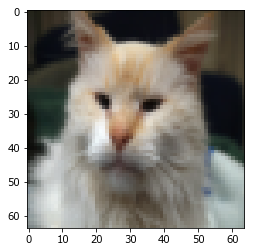：![cat](https://img-blog.csdnimg.cn/20200725113600793.png#pic_center)
2）学习率为0.05时的损失函数：
![cost](https://img-blog.csdnimg.cn/2020072511372295.png?x-oss-process=image/watermark,type_ZmFuZ3poZW5naGVpdGk,shadow_10,text_aHR0cHM6Ly9ibG9nLmNzZG4ubmV0L1B5dGhvbl9tYWRtYW4=,size_16,color_FFFFFF,t_70#pic_center)
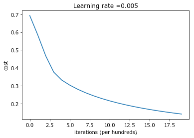
损失一直在下降，说明系统一直在进行改进学习。
3）比较不同学习率条件下的损失函数：
![cost](https://img-blog.csdnimg.cn/20200725113858618.png?x-oss-process=image/watermark,type_ZmFuZ3poZW5naGVpdGk,shadow_10,text_aHR0cHM6Ly9ibG9nLmNzZG4ubmV0L1B5dGhvbl9tYWRtYW4=,size_16,color_FFFFFF,t_70#pic_center)
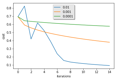
从图片可看出学习率高时最后达到的损失值越低，其中经过多次震荡达到平衡。