BERT+CRF实现中文命名实体识别（TensorFlow）

本篇解读了基于BERT+CRF做中文NER这篇文章中的代码，在该篇作者的GitHub上可以下载源码：源代码。这段代码对BERT模型的实现较为简洁，删掉了谷歌源代码中我们可能用不到的部分，保留了核心部分。对于那些想要快速上手BERT的同学是非常好的学习机会，在看懂这个之后再去学习谷歌的源代码会更加轻松，本篇将尽量详细的对代码进行解读，看完之后如果有合适的数据集就可以自己运行起来了，建议先从原作者的GitHub上把代码下载下来对照着看，数据集也包含在其中。

---

BERT-CRF模型

之前有写过BERT模型和CRF模型的详解，建议往下看之前一定一定要了解这两个模型的原理和工作过程：结合原理和代码来理解bert模型、结合原理与代码理解BiLSTM-CRF模型（pytorch），因为本篇对代码的解读较为详细，如果不清楚BERT模型的原理和工作过程，可能有些地方会很晕。在结合原理和代码来理解bert模型这篇中我也是解读了一个pytorch实现的BERT代码，那段代码更加简洁，只实现了BERT的核心部分，本篇解读的代码基于TensorFlow，会更加接近谷歌的源码。

BERT-CRF与BiLSTM-CRF模型较为相似，其本质上还是一个CRF模型，只不过是用BERT模型来训练CRF模型中的发射矩阵。这个发射矩阵可以用BILSTM来训练，也可以随机初始化训练，但是实际效果都没有BERT好。我自己的NER数据有10多个实体类别，5000个句子，使用这段代码来训练，最终准确度大概为96%。本篇将会把重点放在BERT模型上，代码保留了谷歌源码中的modeling.py、optimization.py、tokenization.py，将run_classifier.py进行了修改，剩下的全部删除，并且调用了谷歌预训练好的模型，接下来会依次介绍代码中的几个模块。

---

Embedding

modeling.py这个文件中定义了BERT模型，主要包括两部分：Embedding和transformer。Embedding用来随机初始化词向量，transformer即BERT模型的主体。

首先介绍与Embedding相关的两个函数：

（1）embedding_lookup

这个函数用来随机生成初始的词向量。函数的参数包括，input_ids：输入序列中每个字在词表中的的索引；vocab_size：词表大小，embedding_size：每个词向量的维度，initializer_range：随机生成正态分布词向量的标准偏差，use_one_hot_embedding：是否使用独热编码。最后返回的是词表中所有词的词向量和输入序列的词向量。

  if input_ids.shape.ndims == 2:
    input_ids = tf.expand_dims(input_ids, axis=[-1])

函数默认输入的是维度为（batch_size，seq_len，input_num）的矩阵，也就是说可以一次输入多个句子。如果只输入了一个句子，即输入矩阵维度为（batch_size，seq_len），那么首先将其维度扩充为（batch_size，seq_len，1）。

  embedding_table = tf.get_variable(
      name=word_embedding_name,
      shape=[vocab_size, embedding_size],
      initializer=create_initializer(initializer_range))

然后使用get_variable函数来初始化词表的词向量，维度为（vocab_size，embedding_size）。初始化的方式在create_initializer方法中，该方法调用了TensorFlow中的truncated_normal_initializer函数，传了一个initializer_range参数，该函数可以生成截断正态分布的初始化矩阵，若某个值超出了initializer_range的范围，则将其丢弃重新生成。

  flat_input_ids = tf.reshape(input_ids, [-1])
  if use_one_hot_embeddings:
    one_hot_input_ids = tf.one_hot(flat_input_ids, depth=vocab_size)
    output = tf.matmul(one_hot_input_ids, embedding_table)
  else:
    output = tf.gather(embedding_table, flat_input_ids)

现在已经有了词表的词向量，我们只需要通过input_ids中的索引，来提取出词向量表中对应位置的词向量即可。首先将input_ids化为一维数组形成索引列表，然后判断是否使用独热编码，在本篇中不使用。gather函数的工作过程就是：将第一个参数看作一张表，第二个参数看成一个索引列表，通过索引来抽取出表中对应位置的数据。这个函数可以帮我们从刚才生成的词向量表中抽取出input_ids位置的词向量，而且此时抽取出的矩阵维度为（batch_size*seq_len，embedding_size），还要将维度进行转换。

  input_shape = get_shape_list(input_ids)
  output = tf.reshape(output, input_shape[0:-1] + [input_shape[-1] * embedding_size])
  return (output, embedding_table)

这两句的目的就是将output转换为（batch_size，seq_len，embedding_size）维度的矩阵。最后返回词向量表和输入序列的词向量。

（2）embedding_postprocessor

这个函数的目的是对上个函数生成的初始词向量做进一步处理，添加序列的type信息和position信息。函数参数包括，input_tensor：输入序列的词向量，也就是上个函数输出的output，use_token_type：是否添加字的type信息，也就是要区分第一句话和第二句话，token_type_ids：输入序列中每个字的type_id，维度是（batch_size，seq_len），也就是预处理时生成的segment_id，第一句为0，第二句为1，token_type_vocab_size：一共有多少种type，这里虽然默认是16，但实际输入的是2，use_position_embeddings：是否添加字的位置信息，initializer_range：权重初始化的范围，与上个函数的该参数作用一致，max_position_embedding：位置Embedding的最大长度，不能比max_seq_len小，dropout_prob：最后输出张量时的丢弃比例。函数返回的还是词向量，与上个函数返回的output维度一致。

  input_shape = get_shape_list(input_tensor, expected_rank=3)
  batch_size = input_shape[0]
  seq_length = input_shape[1]
  width = input_shape[2]

  output = input_tensor

首先把输入矩阵的维度取出来，方便下一步操作。

  if use_token_type:
    if token_type_ids is None:
      raise ValueError("`token_type_ids` must be specified if"
                       "`use_token_type` is True.")
    token_type_table = tf.get_variable(
        name=token_type_embedding_name,
        shape=[token_type_vocab_size, width],
        initializer=create_initializer(initializer_range))
    # This vocab will be small so we always do one-hot here, since it is always
    # faster for a small vocabulary.
    flat_token_type_ids = tf.reshape(token_type_ids, [-1])
    one_hot_ids = tf.one_hot(flat_token_type_ids, depth=token_type_vocab_size)
    token_type_embeddings = tf.matmul(one_hot_ids, token_type_table)
    token_type_embeddings = tf.reshape(token_type_embeddings,
                                       [batch_size, seq_length, width])
    output += token_type_embeddings

如果要添加字的type信息，首先要对两种type_id（0,1）进行初始化编码，得到的token_type_table维度为（2,768）。然后将输入的token_type_ids变化为一维的（batch_size*seq_len），此时生成的flat_token_type_ids中只有0和1，表示每个字的type_id。此时将其生成独热编码，实际上是对0和1进行独热编码，0编码为（1,0）、1编码为（0,1），生成的one_hot_ids维度为（batch_size*seq_len，2）。然后one_hot_ids和token_type_table相乘，就可以得到每个词对应的type_id的编码，维度为（batch_size*seq_len，768）。这里非常巧妙地使用了独热编码来加速运算，建议好好思考一下。最后将type_id信息加到词向量中，进行下一步添加位置信息。

  if use_position_embeddings:
    assert_op = tf.assert_less_equal(seq_length, max_position_embeddings)
    with tf.control_dependencies([assert_op]):
      full_position_embeddings = tf.get_variable(
          name=position_embedding_name,
          shape=[max_position_embeddings, width],
          initializer=create_initializer(initializer_range))

      position_embeddings = tf.slice(full_position_embeddings, [0, 0],
                                     [seq_length, -1])
      num_dims = len(output.shape.as_list())

      # Only the last two dimensions are relevant (`seq_length` and `width`), so
      # we broadcast among the first dimensions, which is typically just
      # the batch size.
      position_broadcast_shape = []
      for _ in range(num_dims - 2):
        position_broadcast_shape.append(1)
      position_broadcast_shape.extend([seq_length, width])
      position_embeddings = tf.reshape(position_embeddings,
                                       position_broadcast_shape)
      output += position_embeddings

如果要添加位置信息，首先对所有位置生成一个初始化向量，维度为（max_position_embeddings，768）。因为我们实际运算时句子长度不会达到max_position_embeddings，所以做个切片操作，只取（seq_length，768）的矩阵即可。然后将这个初始化向量的维度扩充为（1，seq_length，768），再与output相加，不同维度的矩阵相加时会先自动扩充成相同维度。

函数末尾对output进行layer_norm和dropout操作，然后返回，这块就不解释了。经过这两个函数，我们就已经得到了BERT模型的第一部分词向量，然后就是transformer部分。

---

Transformer

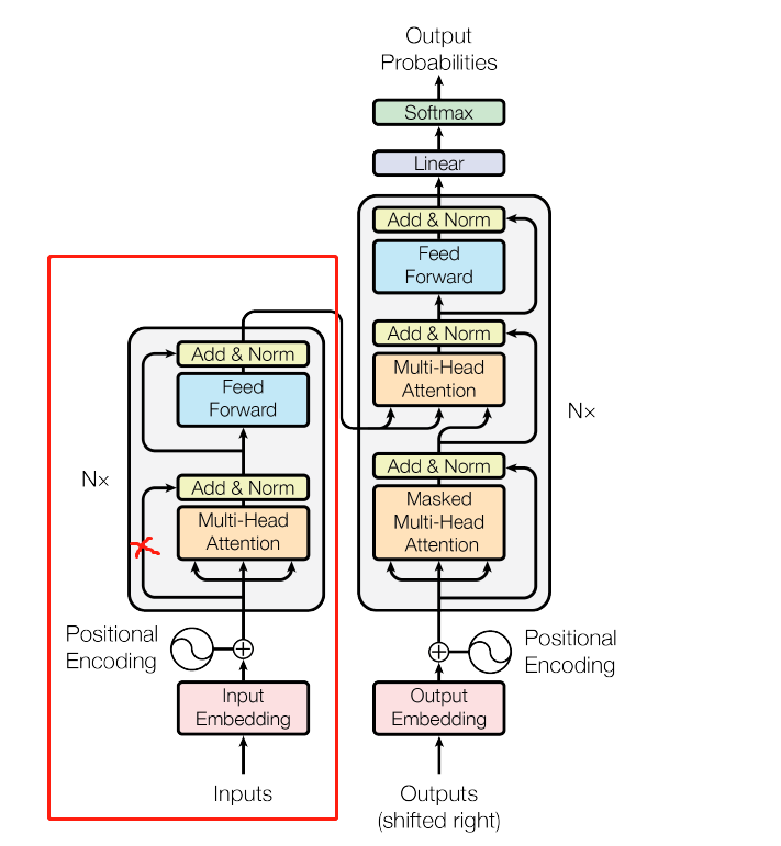
这部分是BERT模型的主体，实际上是transformer中的Encoder，在modeling.py文件定义了两个方法attention_layer和transformer_layer，实现了transformer结构，下面介绍这两个方法。

（1）attention_layer

这个函数主要实现了Encoder中Multi-Head-Attention的部分，主要参数如下，from_tensor，to_tensor：这两个参数是输入的词向量，在我们的程序中是相同的，表示self-Attention。attention_mask：标注序列中哪些位置是无效的pad，不需要参与计算。num_attention_head表表示self-Attention的个数，多个self-Attention组合成最终输出。size_per_head：表示每个self-Attention要处理的向量维数，也就是特征数。query_act、ket_act、value_act：表示Q、K、V矩阵的激活函数。attention_probs_dropout_prob：表示dropout的比例。initializer_range：表示初始化向量的范围。do_return_2d_tensor：是否返回2维的tensor，如果是则返回（batch_size*from_seq_length，num_attention_head*size_per_head）的矩阵。

nun_attention_head乘size_per_head一定是768，所以可以看出每个self-Attention都承担了一部分的词向量，最后再组合成完整的768维词向量。

函数的开头定义了一个函数，transpose_for_score，这个函数用于将输入矩阵的维度从（batch_size*seq_len，768）转换为（batch_size，seq_len，num_attention_head，size_per_head），然后再转换为（batch_size，num_attention_head，seq_len，size_per_head）。这个函数实现比较简单，容易理解。之后获取了两个输入矩阵的维度，并做了一些异常处理。

  from_tensor_2d = reshape_to_matrix(from_tensor)
  to_tensor_2d = reshape_to_matrix(to_tensor)

  # `query_layer` = [B*F, N*H]
  query_layer = tf.layers.dense(
      from_tensor_2d,
      num_attention_heads * size_per_head,
      activation=query_act,
      name="query",
      kernel_initializer=create_initializer(initializer_range))

将输入的两个矩阵转换为二维矩阵，之后使用dense函数定义了Q、K、V矩阵，这里的QKV矩阵维度为（batch_size*seq_len，768）。

  query_layer = transpose_for_scores(query_layer, batch_size, num_attention_heads, from_seq_length, size_per_head)
  key_layer = transpose_for_scores(key_layer, batch_size, num_attention_heads, to_seq_length, size_per_head)

然后将Q、K矩阵的维度变换为（batch_size，num_attention_head，from_seq_len，size_per_head），也就是将768维的词向量分给多个self-Attention来处理，最后结合到一起。

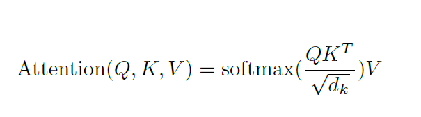
  attention_scores = tf.matmul(query_layer, key_layer, transpose_b=True)
  attention_scores = tf.multiply(attention_scores, 1.0 / math.sqrt(float(size_per_head)))

这里也是常规操作了，公式如下：

  if attention_mask is not None:
    attention_mask = tf.expand_dims(attention_mask, axis=[1])
    adder = (1.0 - tf.cast(attention_mask, tf.float32)) * -10000.0
    attention_scores += adder
  attention_probs = tf.nn.softmax(attention_scores)

在进行softmax操作前，要判断是否要丢弃掉补pad的位置，将补pad位置的得分设置为一个很小的负数，而不是pad的位置就设置为0，这样在softmax时可以消除影响。

attention_probs = dropout(attention_probs, attention_probs_dropout_prob)
  value_layer = tf.reshape(
      value_layer,
      [batch_size, to_seq_length, num_attention_heads, size_per_head])
  value_layer = tf.transpose(value_layer, [0, 2, 1, 3])
  context_layer = tf.matmul(attention_probs, value_layer)

在进行drop操作之后，将V矩阵做与Q、K矩阵相同的维度变换，然后相乘得到Attention_score，这样就完成了上面公式中的全部内容。接下来就是将结果的维度变换回（batch_size，seq_len，768）的形式，然后返回即可。

（2）transformer_model

这个函数调用了上面定义好的Multi-Head-Attention，封装好了transformer结构。主要参数如下，input_tensor：输出的初始词向量。attention_mask：输入序列的mask信息，即标出了哪些位置是无效的pad。hidden_size：词向量的维度。num_hidden_layer：模型中所包含的Encoder的个数。num_attention_head：一个Encoder中self-Attention的个数。intermediate_size：全连接层的维度，就是feedforward那部分。intermediate_act_fn：全连接层使用的激活函数。do_return_all_layer：是否返回每一层Encoder输出的结果。函数返回的是transformer最后一层的输出，维度为（batch_size，seq_len，768）。

函数首先做了一下异常处理和变量的初始化。然后开始计算每一层Encoder的输出。

  prev_output = reshape_to_matrix(input_tensor)

  all_layer_outputs = []
  for layer_idx in range(num_hidden_layers):
    with tf.variable_scope("layer_%d" % layer_idx):
      layer_input = prev_output

从这里我们可以看出，每一层Encoder输入的都是一个二维矩阵，第一层Encoder都使用初始词向量，之后每层使用的是上一层的输出词向量，并且每一层的输出都保存了下来。

        with tf.variable_scope("self"):
          attention_head = attention_layer(
              from_tensor=layer_input,
              to_tensor=layer_input,
              attention_mask=attention_mask,
              num_attention_heads=num_attention_heads,
              size_per_head=attention_head_size,
              attention_probs_dropout_prob=attention_probs_dropout_prob,
              initializer_range=initializer_range,
              do_return_2d_tensor=True,
              batch_size=batch_size,
              from_seq_length=seq_length,
              to_seq_length=seq_length)
          attention_heads.append(attention_head)
        attention_output = None
        if len(attention_heads) == 1:
          attention_output = attention_heads[0]
        else:

          attention_output = tf.concat(attention_heads, axis=-1)

这一部分就是将得到Multi-Head-Attention的输出，虽然代码中定义了一个列表，但实际上我们只输入一个序列，列表中也一直都只有一个矩阵，所以可以忽略那个列表和拼接操作。

        with tf.variable_scope("output"):
          attention_output = tf.layers.dense(
              attention_output,
              hidden_size,
              kernel_initializer=create_initializer(initializer_range))
          attention_output = dropout(attention_output, hidden_dropout_prob)
          attention_output = layer_norm(attention_output + layer_input)

接下来对Multi-Head-Attention的输出进行了线性投影，一个全连接层，再做dropout、残差连接、归一化，也是常规操作了。

      with tf.variable_scope("intermediate"):
        intermediate_output = tf.layers.dense(
            attention_output,
            intermediate_size,
            activation=intermediate_act_fn,
            kernel_initializer=create_initializer(initializer_range))

接下来又连接了一个全连接层，即feedforward部分，在这里中768维的词向量被映射到了更高维度上（3072）。

      with tf.variable_scope("output"):
        layer_output = tf.layers.dense(
            intermediate_output,
            hidden_size,
            kernel_initializer=create_initializer(initializer_range))
        layer_output = dropout(layer_output, hidden_dropout_prob)
        layer_output = layer_norm(layer_output + attention_output)
        prev_output = layer_output
        all_layer_outputs.append(layer_output)

最后就是继续全连接层，映射回768维，然后dropout、残差连接、归一化，得到本层Encoder的输出，更新输入词向量，保存结果，也是常规操作了。结合下面Encoder层的结构图应该可以更好地理解这一过程：

到这里BERT模型的两大部分就定义完了，接下来我们就该实现BERT模型的配置和组装了。

---

BERT

BERT模型的构建主要是由modeling.py文件中BertModel类和BertConfig类完成的。其中BertConfig类中实现了读取BERT模型配置文件的方法，并且初始化了BERT模型的参数，就不多讲了。

BertModel类读取了BertConfig类中初始化的模型参数，接收输入的序列信息，类的重点在其初始化函数中，初始化函数组装了上面讲的两大部分，获取到了最终的输出。类中初始化函数的主要参数如下，config：模型的配置参数。is_training：是否在训练状态。nput_ids：输入序列中的字在此表中的索引，维度为（batch_size，seq_len）。input_mask：输入序列中要mask的位置，即不需要参与计算的位置。token_type_ids：输入序列的type信息。函数最后得到了transformer的输出，和每个序列中第一个词的输出，也就是CLS的词向量，可以用来进行文本分类。函数开头的一些初始化操作就不再提了，直接进入正题。

      with tf.variable_scope("embeddings"):
        (self.embedding_output, self.embedding_table) = embedding_lookup(
            input_ids=input_ids,
            vocab_size=config.vocab_size,
            embedding_size=config.hidden_size,
            initializer_range=config.initializer_range,
            word_embedding_name="word_embeddings",
            use_one_hot_embeddings=use_one_hot_embeddings)
        self.embedding_output = embedding_postprocessor(
            input_tensor=self.embedding_output,
            use_token_type=True,
            token_type_ids=token_type_ids,
            token_type_vocab_size=config.type_vocab_size,
            token_type_embedding_name="token_type_embeddings",
            use_position_embeddings=True,
            position_embedding_name="position_embeddings",
            initializer_range=config.initializer_range,
            max_position_embeddings=config.max_position_embeddings,
            dropout_prob=config.hidden_dropout_prob)

与我介绍的顺序一致，函数中首先对输入序列生成了初始化词向量，对词向量做了补充操作，添加了type信息和位置信息，传入的参数只要能明白作用是什么就好。这段中我们得到了初始词向量self.embedding_output。

      with tf.variable_scope("encoder"):
        attention_mask = create_attention_mask_from_input_mask(
            input_ids, input_mask)
        self.all_encoder_layers = transformer_model(
            input_tensor=self.embedding_output,
            attention_mask=attention_mask,
            hidden_size=config.hidden_size,
            num_hidden_layers=config.num_hidden_layers,
            num_attention_heads=config.num_attention_heads,
            intermediate_size=config.intermediate_size,
            intermediate_act_fn=get_activation(config.hidden_act),
            hidden_dropout_prob=config.hidden_dropout_prob,
            attention_probs_dropout_prob=config.attention_probs_dropout_prob,
            initializer_range=config.initializer_range,
            do_return_all_layers=True)

接着调用了transformer结构，使用刚才生成的self.embedding_output作为输入，得到了每一层Encoder的输出。其他参数能看懂作用是什么就行，注意这里do_return_all_layers设置为True。至于create_attention_mask_from_input_mask这个名字巨长的函数，可以不看，想想就知道是要生成mask矩阵。这段我们得到了transformer中每一层的输出self.all_encoder_layers。

      self.sequence_output = self.all_encoder_layers[-1]

这句话用来提取出transformer最后一层的输出，也就是BERT模型的输出词向量，定义为self.sequence_output。

      with tf.variable_scope("pooler"):
        first_token_tensor = tf.squeeze(self.sequence_output[:, 0:1, :], axis=1)
        self.pooled_output = tf.layers.dense(
            first_token_tensor,
            config.hidden_size,
            activation=tf.tanh,
            kernel_initializer=create_initializer(config.initializer_range))

这段的作用就是刚才所说的，提取出每个句子中第一个位置CLS的词向量，因为经过transformer后，CLS中包含了整个句子的信息，可以用它来进行句子级的分类任务。这里的self.pooled_output的维度为（batch_size，768）。

到这里整个BERT模型的构建就完成了，modeling.py文件中的内容也介绍的差不多了，接下来就该到run_ner.py文件中准备数据，训练模型，实现NER了。

---

准备数据

代码中有一个tokenizer.py文件，其中定义了许多处理原始数据的方法，包括大小写转换、Unicode转换、token和id的索引。这个文件中的代码还是较为容易理解的，有一定的python基础就能看懂，在用的时候只需要知道输入输出是什么就可以了。

数据准备还涉及到run_ner文件中多个类和方法，下面逐个介绍。首先看一下训练集和测试集的格式：

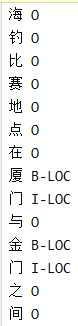
每行对应一个字及其分类，一个空行表示一个句子的结束。我们将会把这种形式的数据进行一步步的处理，最终生成适用于模型的输入数据，下面介绍从原始数据到模型输入数据的处理过程

（1）NerProcessor类

这个类主要就是定义了读取训练集、测试集和标签集的方法，这三个方法本身较为简单，调用了DataProcessor类中的read_data方法也容易理解。类中还定义了一个create_example方法，调用了InputExample类来将一个句子的字序列和标签序列封装起来。InputExample类包含了一个句子的ID、子序列、标签序列：

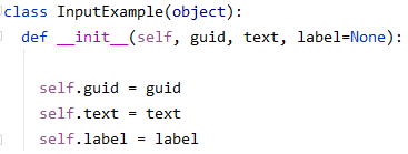
所以这个类的作用就是，将训练集和测试集中的每个句子都封装成一个InputExample实例，然后返回。这个类的实现较为简单，我们只需要知道处理完之后的数据格式即可，例如：

（2）convert_single_example

这个方法用于将一个InputExample类的数据转换为一个InputFeature类的数据。函数的主要参数如下，ex_index：当前这个InputExample的索引。example：当前传入的一个InputExample实例。label_list：所有标签的集合。max_seq_len：句子的最大长度，其实也就是要把所有句子统一到这个长度。tokenizer：原始数据解析器。函数返回一个InputFeature实例。

InputFeature类的属性包含句子的各种信息，接下来我们就要对InputExample实例进行解析，得到下面这些属性：

    label_map = {}
    for (i,label) in enumerate(label_list):
        label_map[label] = i

    with open(FLAGS.output_dir+"/label2id.pkl",'wb') as w:
        pickle.dump(label_map,w)

函数首先给所有标签设置了一个索引，然后将这个map形式的标签集保存到文件中，方便之后调用。

    textlist = example.text.split(' ')
    labellist = example.label.split(' ')#在这里进行切分，之前都是字符串
    tokens = []
    labels = []
    for i,(word,label) in enumerate(zip(textlist,labellist)):
        tokens.append(word)
        labels.append(label)

因为在InputExample中，token和label是将每个字或标签用空格连接形成的字符串，所以函数要将一个InputExample中的token和label进行切分，得到一个列表形式的token和label。此时的tokens中保存的是一句话中的每个字，labels中保存的是一句话中每个字的标签。

    ntokens.append("[CLS]")
    segment_ids.append(0)
    label_ids.append(label_map["[CLS]"])
    for i, token in enumerate(tokens):
        ntokens.append(token)
        segment_ids.append(0)
        label_ids.append(label_map[labels[i]])
    
    input_ids = tokenizer.convert_tokens_to_ids(ntokens)
    mask = [1]*len(input_ids)

在这里给每句话添加了CLS，且NER问题不需要两句话的拼接，所以也用不到SEP。添加CLS后，segment_ids序列中也要加上CLS对应的0。这个for循环生成了句子最终的token序列、segment_ids、label_ids。接着调用了tokenizer中的一个方法，这个方法其实也不用去细看，只需要知道他根据生成的token序列返回了句子的input_ids即可。mask序列也就可以根据input_ids的长度来填充1了。

    while len(input_ids) < max_seq_length:
        input_ids.append(0)
        mask.append(0)
        segment_ids.append(0)
        label_ids.append(0)#label_map["[PAD]"]==0
        ntokens.append("[PAD]")

紧接着为了统一句子长度，给每个长度不足max_seq_len的句子末尾填充一些0。到这里，InputFeature类所需要的信息都已经准备好了，最后封装起来返回即可，格式大致如下，长度不足的后面全补了0。

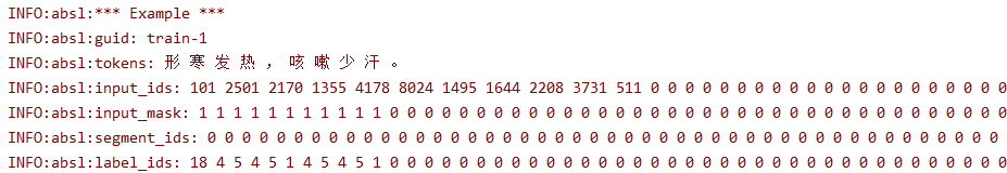
（2）filled_based_convert_examples_to_features

这个方法调用了上面的convert_single_example方法，先将所有InputExample类数据转换为InputFeature类数据，然后转换为为TensorFlow中特有的Example型数据，最后保存到tf_record型文件中。tf_record文件是TensorFlow推荐使用的一种二进制文件，理论上可以保存任何数据。

函数的主要参数如下：examples：所有的InputExample类数据。label_list：数据集中存在的所有标签类别。max_seq_len：句子的最大长度。tokenizer：数据预处理的解析器。output_file：生成的tf_record文件保存的位置。

        def create_int_feature(values):
            f = tf.train.Feature(int64_list=tf.train.Int64List(value=list(values)))
            return f

在函数中定义的这个create_int_feature函数是核心内容，他接收了一个列表，并将其转换为TensorFlow中的Feature型数据。首先，tf.train.Int64List(value=list(values))将列表转换为了“value：data”形式的数据，例如：

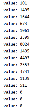
然后tf.train.Feature(int64_list=tf.train.Int64List(value=list(values)))将上面的“value：data”形式的数据封装起来，看作是一个特征集，变成下面这个样子：

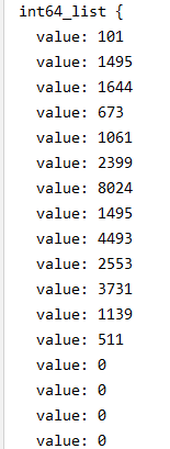
        features = collections.OrderedDict()
        features["input_ids"] = create_int_feature(feature.input_ids)
        features["mask"] = create_int_feature(feature.mask)
        features["segment_ids"] = create_int_feature(feature.segment_ids)
        features["label_ids"] = create_int_feature(feature.label_ids)

这里就是在给每个信息构建特征集，features是一个字典，而且其中元素的顺序与输入的顺序一致。现在我们得到了特征名到特征集的字典，然后就可以将他们组合起来，创建一个多种类型的特征集，即多个feature的集合。

        tf_example = tf.train.Example(features=tf.train.Features(feature=features))

首先tf.train.Features(feature=features)会将多个Feature型的数据组合成一个Features型的数据，然后再调用Example模块形成一个Example形式的数据。

处理过程总结一下就是：list -> Int64List -> Feature -> Features -> Example。多输出几次中间变量就可以明白这个过程了。

        writer.write(tf_example.SerializeToString())

在最后将这个Example型数据转换为字符串写入文件中即可。

到这里数据准备就已经完成了，接下来就是调用输入函数进行训练即可，每次向模型中输入一个batch的数据。