论文翻译《Cascade R-CNN: Delving into High Quality Object Detection》

论文地址：https://arxiv.org/abs/1712.00726
代码地址：https://github.com/zhaoweicai/cascade-rcnn

Abstract

In object detection, an intersection over union (IoU) threshold is required to define positives and negatives. An object detector, trained with low IoU threshold, e.g. 0.5, usually produces noisy detections. However, detection performance tends to degrade with increasing the IoU thresholds. Two main factors are responsible for this: 1) overfitting during training, due to exponentially vanishing positive samples, and 2) inference-time mismatch between the IoUs for which the detector is optimal and those of the input hypotheses. A multi-stage object detection architecture,the Cascade R-CNN, is proposed to address these problems. It consists of a sequence of detectors trained with increasing IoU thresholds, to be sequentially more selective against close false positives. The detectors are trained stage by stage, leveraging the observation that the output of a detector is a good distribution for training the next higher quality detector. The resampling of progressively improved hypotheses guarantees that all detectors have a positive set of examples of equivalent size, reducing the overfitting problem. The same cascade procedure is applied at inference, enabling a closer match between the hypotheses and the detector quality of each stage. A simple implementation of the Cascade R-CNN is shown to surpass all single-model object detectors on the challenging COCO dataset. Experiments also show that the Cascade R-CNN is widely applicable across detector architectures, achieving consistent gains independently of the baseline detector strength. The code will be made available at https://github.com/zhaoweicai/cascade-rcnn.

在目标检测中，需要一个交并比（IoU）阈值来定义阳性和假阳性。用低IoU阈值（例如0.5）训练的目标检测器通常会产生噪声检测。但是，随着IoU阈值的增加，检测性能往往趋于下降。造成这种情况的两个主要因素是:1）训练期间的过拟合，由于正样本的指数消失；2）检测器最优的IoU与输入建议框之间的推断时间不匹配。为了解决这些问题，提出了一种多级目标检测体系结构Cascade R-CNN。它由一系列检测器组成，这些检测器经过不断增加的IoU阈值训练，从而对接近的假阳性有更强的选择性。检测器是分阶段训练的，一个高质量的检测器的输出用于训练下一个更高质量的检测器。逐步改进的建议框的重新采样保证了所有检测器都有一个大小相当的正样本集，减少了过拟合问题。推理时采用相同的级联过程，使预测结果和每个阶段的检测器质量之间的更紧密匹配。Cascade R - CNN的简单实现在具有挑战性的COCO数据集上超过了所有单模型目标检测器。实验还表明，Cascade R-CNN广泛适用于检测器架构，实现独立于基线检测器强度的一致增益。代码将在https://github.com/zhaoweicai/cascade-rcnn上提供。

1. Introduction

Object detection is a complex problem, requiring the solution of two main tasks. First, the detector must solve the recognition problem, to distinguish foreground objects from background and assign them the proper object class labels. Second, the detector must solve the localization problem, to assign accurate bounding boxes to different objects. Both of these are particularly difficult because the detector faces many “close” false positives, corresponding to “close but not correct” bounding boxes. The detector must find the true positives while suppressing these close false positives.

目标检测是一个复杂的问题，需要解决两个主要任务。首先，检测器必须解决识别问题，将前景物体与背景区分开来，并为其分配合适的对象类标签。其次，检测器必须解决定位问题，为不同对象分配精确的边界框。这两者都特别困难，因为检测器面临许多"接近"的假阳性，对应于"接近但不正确"的边界框。检测器必须在抑制这些接近的假阳性的同时找到真正的阳性。

Many of the recently proposed object detectors are based on the two-stage R-CNN framework [12, 11, 27, 21], where detection is framed as a multi-task learning problem that combines classification and bounding box regression. Unlike object recognition, an intersection over union (IoU) threshold is required to define positives/negatives. However, the commonly used threshold values u, typically $u=0.5$, establish quite a loose requirement for positives. The resulting detectors frequently produce noisy bounding boxes, as shown in Figure 1 (a). Hypotheses that most humans would consider close false positives frequently pass the IoU ≥ 0.5 test. While the examples assembled under the $u=0.5$ criterion are rich and diversified, they make it difficult to train detectors that can effectively reject close false positives.

最近提出的许多目标检测器都是基于两阶段的R - CNN框架[ 12、11、27、21]，其中检测被定义为一个结合分类和边界框回归的多任务学习问题。与对象识别不同，需要一个交并( IoU )阈值来定义正/负。然而，常用的阈值$u$，通常是$u=0.5$，对判定为正样本的要求相当宽松。由此产生的检测器经常产生有噪声的边界框，如图1 ( a )所示。大多数人认为“接近假阳性”的建议框经常通过IoU≥0.5检验。虽然在$u=0.5$准则下组装的示例丰富多样，但它们很难训练出能够有效拒绝“接近假阳性”的检测器。

In this work, we define the quality of an hypothesis as its IoU with the ground truth, and the quality of the detector as the IoU threshold u used to train it. The goal is to investigate the, so far, poorly researched problem of learning high quality object detectors, whose outputs contain few close false positives, as shown in Figure 1 (b). The basic idea is that a single detector can only be optimal for a single quality level. This is known in the cost-sensitive learning literature [7, 24], where the optimization of different points of the receiver operating characteristic (ROC) requires different loss functions. The main difference is that we consider the optimization for a given IoU threshold, rather than false positive rate.

在这项工作中，我们定义建议框的质量为其与真实值的IoU，并将检测器的质量定义为用于训练它的IoU阈值。目标是研究迄今为止研究较少的学习高质量目标检测器的问题，其输出包含少量接近的假阳性，如图1 ( b )所示。其基本思想是：单个检测器只能对单一质量水平最优。这在代价敏感学习文献[ 7、24]中已知，其中接受机工作特性(receiver operating characteristic, ROC)的不同点需要不同的损失函数。主要区别在于我们考虑的是优化给定的IoU阈值，而不是优化假阳性率。

The idea is illustrated by Figure 1 © and (d), which present the localization and detection performance, respectively, of three detectors trained with IoU thresholds of $u=0.5,0.6,0.7$. The localization performance is evaluated as a function of the IoU of the input proposals, and the detection performance as a function of IoU threshold, as in COCO [20]. Note that, in Figure 1 ©, each bounding box regressor performs best for examples of IoU close to the threshold that the detector was trained. This also holds for detection performance, up to overfitting. Figure 1 (d) shows that, the detector of $u=0.5$ outperforms the detector of $u=0.6$ for low IoU examples, underperforming it at higher IoU levels. In general, a detector optimized at a single IoU level is not necessarily optimal at other levels. These observations suggest that higher quality detection requires a closer quality match between the detector and the hypotheses that it processes. In general, a detector can only have high quality if presented with high quality proposals.

图1 ( c )和(d)说明了这一思想，图1 ( c )和(d)分别展示了用$u=0.5、0.6、0.7$的IoU阈值训练的三个检测器的定位和检测性能。定位性能用于评估输入建议框的IoU，检测性能用于评估IoU阈值，如COCO[20]。请注意，在图1 ( c )中，只有建议框自身的阈值和训练器训练用的阈值较为接近的时候，训练器的性能才最好。这也适用于检测性能，直到过拟合。图1 (d)显示，$u=0.5$在低IoU的情况下优于$u=0.6$的检测器，在高IoU的情况下表现较差。通常，在单个IoU级别上优化的检测器在其他级别上不一定是最优的。这些观察表明，更高质量的检测需要检测器与其处理的建议框之间更紧密的质量匹配。一般来说，只有在提供高质量的建议框时，检测器才能具有高质量。

However, to produce a high quality detector, it does not suffice to simply increase u during training. In fact, as seen for the detector of $u=0.7$ of Figure 1 (d), this can degrade detection performance. The problem is that the distribution of hypotheses out of a proposal detector is usually heavily imbalanced towards low quality. In general, forcing larger IoU thresholds leads to an exponentially smaller numbers of positive training samples. This is particularly problematic for neural networks, which are known to be very example intensive, and makes the “high u” training strategy quite prone to overfitting. Another difficulty is the mismatch between the quality of the detector and that of the testing hypotheses at inference. As shown in Figure 1, high quality detectors are only necessarily optimal for high quality hypotheses. The detection could be suboptimal when they are asked to work on the hypotheses of other quality levels.

然而，要搭建一个高质量的检测器，仅仅在训练时增加u是不够的。事实上，如图1 ( d )中$u=0.7$的检测器所示，这会降低探测性能。问题是区域建议框检测器输出的建议框分布通常严重不平衡，趋向于低质量。一般来说，强行增大IoU阈值会导致正训练样本的数量呈指数下降。这对于众所周知的样本非常密集的神经网络来说尤其有问题，并且使得"高u "训练策略相当容易出现过拟合。另一个困难是检测器的质量与测试时检验建议框的质量不匹配。如图1所示，高质量的检测器只对高质量的建议框是最优的。当要求他们在其他质量水平的建议框上工作时，检测可能是次优的。

In this paper, we propose a new detector architecture, Cascade R-CNN, that addresses these problems. It is a multi-stage extension of the R-CNN, where detector stages deeper into the cascade are sequentially more selective against close false positives. The cascade of R-CNN stages are trained sequentially, using the output of one stage to train the next. This is motivated by the observation that the output IoU of a regressor is almost invariably better than the input IoU. This observation can be made in Figure 1 ( c ), where all plots are above the gray line. It suggests that the output of a detector trained with a certain IoU threshold is a good distribution to train the detector of the next higher IoU threshold.

在本文中，我们提出了一种新的检测器体系结构，Cascade R-CNN，以解决这些问题。它是R-CNN的多级扩展，其中级联更深的检测器阶段对“接近假阳性”的选择性更强。级联的R-CNN阶段按顺序训练，使用一个阶段的输出来训练下一个阶段。这是由于观察到回归的输出IoU几乎总是比输入IoU好。这种观察可以在图1 ( c )中得到，其中所有的图都在灰色线以上。这表明，用某个IoU阈值训练的检测器的输出是一个很好的分布，可以训练下一个更高IoU阈值的检测器。

This is similar to boostrapping methods commonly used to assemble datasets in object detection literature [31, 8]. The main difference is that the resampling procedure of the Cascade R-CNN does not aim to mine hard negatives. Instead, by adjusting bounding boxes, each stage aims to find a good set of close false positives for training the next stage. When operating in this manner, a sequence of detectors adapted to increasingly higher IoUs can beat the overfitting problem, and thus be effectively trained. At inference, the same cascade procedure is applied. The progressively improved hypotheses are better matched to the increasing detector quality at each stage.This enables higher detection accuracies, as suggested by Figure 1 ( c )and (d).

这类似于物体检测文献[31,8]中通常用于组装数据集的boostrapping方法。主要的区别是Cascade R-CNN的重采样过程并不旨在挖掘困难负样本（即假阳性）。相反，通过调整边界框，每个阶段都旨在为下一阶段的训练找到一组良好的“接近假阳性”。当以这种方式操作时，检测器序列可以适应越来越高的IoU，从而克服过拟合问题，进行有效地训练。在测试时，采用相同的级联过程。逐步改进的建议框与每个阶段不断提高的检测器质量更好地匹配，这可以实现更高的检测精度，如图1 ( c )和(d)所示。

The Cascade R-CNN is quite simple to implement and trained end-to-end. Our results show that a vanilla implementation, without any bells and whistles, surpasses all previous state-of-the-art single-model detectors by a large margin, on the challenging COCO detection task [20], especially under the higher quality evaluation metrics. In addition, the Cascade R-CNN can be built with any two-stage object detector based on the R-CNN framework. We have observed consistent gains (of 2∼4 points), at a marginal increase in computation. This gain is independent of the strength of the baseline object detectors. We thus believe that this simple and effective detection architecture can be of interest for many object detection research efforts.

Cascade R - CNN非常简单，可以端到端的实现和训练。我们的结果表明，在具有挑战性的COCO检测任务[20]上，特别是在更高质量的评估指标下，一个没有任何花哨功能的普通实现，大大超过了所有以前最先进的单模型探测器。此外，Cascade R-CNN可以使用基于R-CNN框架的任何两级对象检测器来构建。我们已经观察到在计算量的边际增加的情况下，获得持续的增益(2 ~ 4个点)。这个增益与基线目标探测器的强度无关。因此，我们相信这种简单而有效的检测体系结构可以引起许多目标检测研究的兴趣。

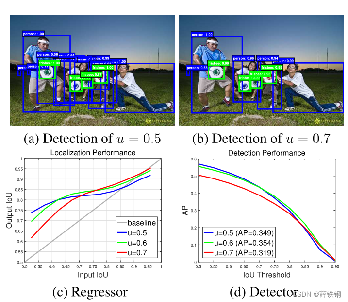
Figure 1. The detection outputs, localization and detection performance of object detectors of increasing IoU threshold u.

图1。提高IoU阈值u后目标探测器的识别、定位和检测性能。

2. Related Work

Due to the success of the R-CNN [12] architecture, the two-stage formulation of the detection problems, by combining a proposal detector and a region-wise classifier has become predominant in the recent past. To reduce redundant CNN computations in the R-CNN, the SPP-Net [15] and Fast-RCNN [11] introduced the idea of region-wise feature extraction, significantly speeding up the overall detector. Later, the Faster-RCNN [27] achieved further speedsup by introducing a Region Proposal Network (RPN). This architecture has become a leading object detection framework. Some more recent works have extended it to address various problems of detail. For example, the R-FCN [4] proposed efficient region-wise fully convolutions without accuracy loss, to avoid the heavy region-wise CNN computations of the Faster-RCNN; while the MS-CNN [1] and FPN [21] detect proposals at multiple output layers, so as to alleviate the scale mismatch between the RPN receptive fields and actual object size, for high-recall proposal detection.

由于R-CNN[12]架构的成功，通过组合一个建议框检测器和一个区域分类器来解决检测问题的两阶段方案已经成为了主流。为了减少R-CNN中的冗余CNN计算，SPP-Net[15]和Fast-RCNN[11]引入了区域特征提取的思想，显著加快了整体检测器的速度。后来，Faster-RCNN[27]通过引入区域建议网络(RPN)实现了进一步的加速。该体系结构已成为领先的目标检测框架。最近的一些工作对其进行了扩展，以解决各种细节问题。例如，R-FCN [ 4 ]提出了高效且不损失精度的区域全卷积，避免了Faster - RCNN中繁重的区域CNN计算；而MS-CNN[1]和FPN[21]在多个输出层检测候选区域，从而缓解RPN感受野与实际物体大小之间的尺度不匹配问题，实现高召回率候选区域检测。

Alternatively, one-stage object detection architectures have also become popular, mostly due to their computational efficiency. These architectures are close to the classic sliding window strategy [31, 8]. YOLO [26] outputs very sparse detection results by forwarding the input image once. When implemented with an efficient backbone network, it enables real time object detection with fair performance. SSD [23] detects objects in a way similar to the RPN [27], but uses multiple feature maps at different resolutions to cover objects at various scales. The main limitation of these architectures is that their accuracies are typically below that of two-stage detectors. Recently, RetinaNet [22] was proposed to address the extreme foreground-background class imbalance in dense object detection, achieving better results than state-of-the-art two-stage object detectors.

此外，单阶段目标检测架构也变得流行起来，这主要是由于它们的计算效率。这些架构都接近经典的滑动窗口策略[ 31、8]。YOLO [ 26 ]通过转发输入图像一次，输出非常稀疏的检测结果。当使用高效的backbone实现时，它能够以公平的性能实现实时目标检测。SSD [ 23 ]以类似于RPN [ 27 ]的方式检测物体，但使用不同分辨率的多个特征映射来覆盖不同尺度的对象。这些结构的主要局限性在于其精度通常低于两阶段探测器。最近，RetinaNet [ 22 ]被提出用于解决密集目标检测中极端的前景-背景类别不平衡问题，取得了比现有的两阶段目标检测器更好的效果。

Some explorations in multi-stage object detection have also been proposed. The multi-region detector [9] introduced iterative bounding box regression, where a R-CNN is applied several times, to produce better bounding boxes. CRAFT [33] and AttractioNet [10] used a multi-stage procedure to generate accurate proposals, and forwarded them to a Fast-RCNN. [19, 25] embedded the classic cascade architecture of [31] in object detection networks. [3] iterated a detection and a segmentation task alternatively, for instance segmentation.

在多级目标检测方面也进行了一些探索。多区域检测器[9]引入迭代边界框回归，其中R - CNN被多次应用，以产生更好的边界框。CRAFT [33]和AttractioNet [10]使用多阶段过程生成精确的建议框，并将其转发到Fast - RCNN。[19、25]在目标检测网络中嵌入了经典的级联结构[31]。[3]交替迭代一个检测任务和一个分割任务，例如实例分割。

3. Object Detection

In this paper, we extend the two-stage architecture of the Faster-RCNN [27, 21], shown in Figure 3 (a). The first stage is a proposal sub-network (“$H0$”), applied to the entire image, to produce preliminary detection hypotheses, known as object proposals. In the second stage, these hypotheses are then processed by a region-of-interest detection sub-network (“$H1$”), denoted as detection head. A final classification score (“$C$”) and a bounding box (“$B$”) are assigned to each hypothesis. We focus on modeling a multi-stage detection sub-network, and adopt, but are not limited to, the RPN [27] for proposal detection.

在本文中，我们扩展了Faster - RCNN的两阶段架构[27,21]，如图3 (a)所示。第一阶段是一个建议子网络(“$H0$”)，应用于整个图像，以产生初步的检测假设，称为目标建议框。在第二阶段，这些建议框被一个感兴趣区域检测子网络(“$H1$”)处理，记为检测头。每个建议框都有一个最终的分类分数(“$C$”)和一个边界框(“$B$”)。我们专注于建模一个多级检测子网络，采用但不限于RPN[27]进行建议检测。

3.1. Bounding Box Regression

A bounding box $b=(b_x,b_y,b_w,b_h)$ contains the four coordinates of an image patch $x$. The task of bounding box regression is to regress a candidate bounding box b into a target bounding box g, using a regressor $f(x,b)$. This is learned from a training sample $g_i,b_i$, so as to minimize the bounding box risk
$$R_{loc}[f]=\sum _{i=1}^N{L}_{loc}(f(x_i,b_i),g_i)\text{\hspace{1em}(1)}$$

边界框$b=(b_x,b_y,b_w,b_h)$包含图像块$x$的四个坐标。边界框回归的任务是使用回归器$f(x,b)$将候选边界框b回归到目标边界框g。这是从训练样本$g_i,b_i$中学习的，从而使边界框风险最小化
$$R_{loc}[f]=\sum _{i=1}^N{L}_{loc}(f(x_i,b_i),g_i)\text{\hspace{1em}(1)}$$

where $L_{loc}$ was a $L_2$ loss function in R-CNN [12], but updated to a smoothed $L_1$ loss function in Fast-RCNN [11]. To encourage a regression invariant to scale and location, $L_{loc}$ operates on the distance vector $\Delta ={\delta }_x,{\delta }_y,{\delta }_w,{\delta }_h$ defined by
$${\delta }_x=(g_x-b_x)/b_w,{\delta }_y=(g_y-b_y)/b_h$$
$${\delta }_w=log(g_w/b_w),{\delta }_h=log(g_h/b_h)\text{\hspace{1em}(2)}$$

其中，$L_{loc}$是R - CNN中的$L_2$损失函数[ 12 ]，但在Fast - RCNN中更新为smooth$L_1$loss损失函数[ 11 ]。为了增加尺度和回归不变性，$L_{loc}$对定义的距离向量$\Delta ={\delta }_x,{\delta }_y,{\delta }_w,{\delta }_h$定义为
$${\delta }_x=(g_x-b_x)/b_w,{\delta }_y=(g_y-b_y)/b_h$$
$${\delta }_w=log(g_w/b_w),{\delta }_h=log(g_h/b_h)\text{\hspace{1em}(2)}$$

Since bounding box regression usually performs minor adjustments on $b$, the numerical values of (2) can be very small. Hence, the risk of (1) is usually much smaller than the classification risk. To improve the effectiveness of multi-task learning, $\Delta$ is usually normalized by its mean and variance, i.e. ${\delta }_x$ is replaced by ${\delta }_x^{{}^{\prime }}=({\delta }_x-{\mu }_x)/{\sigma }_w$. This is widely used in the literature [27, 1, 4, 21, 14].

由于边界框回归通常对$b$进行微小的调整，因此( 2 )式的数值可能很小。因此，( 1 )的风险通常比分类风险小得多。为了提高多任务学习的有效性，$\Delta$通常用其均值和方差进行归一化，即将${\delta }_x$替换为${\delta }_x^{{}^{\prime }}=({\delta }_x-{\mu }_x)/{\sigma }_w$。这在文献[ 27、1、4、21、14]中被广泛使用。

Some works [9, 10, 16] have argued that a single regression step of $f$ is insufficient for accurate localization. Instead, $f$ is applied iteratively, as a post-processing step
$$f^{{}^{\prime }}(x,b)=fofo...of(x,b)\text{\hspace{1em}(3)}$$
to refine a bounding box b. This is called iterative bounding box regression, denoted as iterative BBox. It can be implemented with the inference architecture of Figure 3 (b) where all heads are the same. This idea, however, ignores two problems. First, as shown in Figure 1, a regressor $f$ trained at $u=0.5$, is suboptimal for hypotheses of higher IoUs. It actually degrades bounding boxes of IoU larger than 0.85. Second, as shown in Figure 2, the distribution of bounding boxes changes significantly after each iteration. While the regressor is optimal for the initial distribution it can be quite suboptimal after that. Due to these problems, iterative BBox requires a fair amount of human engineering, in the form of proposal accumulation, box voting, etc. [9, 10, 16], and has somewhat unreliable gains. Usually, there is no benefit beyond applying f twice.

一些工作[ 9、10、16]认为，$f$的单一回归步骤不足以准确定位。取而代之的是迭代运用$f$，作为后处理步骤
$$f^{{}^{\prime }}(x,b)=fofo...of(x,b)\text{\hspace{1em}(3)}$$
这称为迭代边界框回归，记为迭代BBox。它可以用图3 ( b )的推理架构来实现，其中所有的头都是相同的。然而，这种思路忽略了两个问题。首先，如图1所示，在$u=0.5$处训练的回归器$f$对于IoU较高的假设是次优的。这实际上是对IoU大于0.85的边界框的降级。其次，如图2所示，边界框的分布在每次迭代后都发生了明显的变化。虽然回归器对初始分布是最优的，但在此之后它可以是相当次优的。由于这些问题，迭代BBox需要相当数量的人工工程，以建议框累加、投票等形式进行。[ 9、10、16]，效果具有一定的不可靠性。通常情况下，除了应用两次f之外没有任何好处。

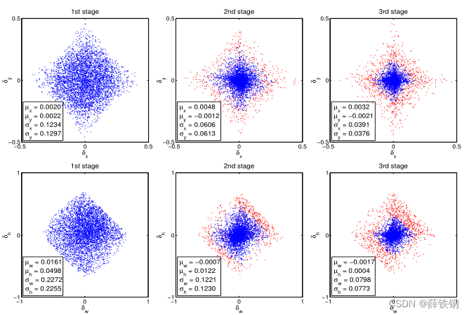
Figure 2. Sequential $\Delta$ distribution (without normalization) at different cascade stage. Red dots are outliers when using increasing
IoU thresholds, and the statistics are obtained after outlier removal.

图2。在不同级联阶段的顺序$\Delta$分布(无归一化)。红点为增加IoU阈值时的离群值，并在去除异常值后得到统计量。

3.2. Classification

The classifier is a function $h(x)$ that assigns an image patch $x$ to one of $M+1$ classes, where class 0 contains background and the remaining the objects to detect. $h(x)$ is a $M+1$-dimensional estimate of the posterior distribution over classes, i.e. $h_k(x)=p(y=k|x)$, where $y$ is the class label. Given a training set $(x_i,y_i)$, it is learned by minimizing a classification risk
$$R_{cls}[h]=\sum _{i=1}^N{L}_{cls}(h(x_i),y_i)\text{\hspace{1em}(4)}$$
where $L_{cls}$ is the classic cross-entropy loss.

分类器是一个函数$h(x)$，将一个图像块x分配给$M+1$类中的一个，其中第0类为背景，其余为待检测对象。$h(x)$是类的后验分布的$M+1$维估计，即$h_k(x)=p(y=k|x)$，其中y为类标签。给定一个训练集$(x_i,y_i)$，通过最小化一个分类风险来学习
$$R_{cls}[h]=\sum _{i=1}^N{L}_{cls}(h(x_i),y_i)\text{\hspace{1em}(4)}$$
其中， $L_{cls}$是典型的交叉熵损失。

3.3. Detection Quality

Since a bounding box usually includes an object and some amount of background, it is difficult to determine if a detection is positive or negative. This is usually addressed by the IoU metric. If the IoU is above a threshold $u$, the patch is considered an example of the class. Thus, the class label of a hypothesis $x$ is a function of $u$,
$$y=\{\begin{array}{rl}{g}_y& ,IoU(x,y)\ge u\\ 0& ,otherwise\end{array}\text{\hspace{1em}(5)}$$
where $g_y$ is the class label of the ground truth object $g$. This
IoU threshold $u$ defines the quality of a detector.

由于边界框通常包含一个物体和一定数量的背景，因此很难确定检测是阳性还是假阳性。这通常通过IoU度量来解决。如果IoU大于某个阈值$u$，则认为该图像块属于该类，是该类的一个实例。因此，假设$x$的类别标签是$u$的函数，
$$y=\{\begin{array}{rl}{g}_y& ,IoU(x,y)\ge u\\ 0& ,otherwise\end{array}\text{\hspace{1em}(5)}$$
其中，$g_y$是ground truth对象$g$的类标签。这个IoU阈值$u$定义了检测器的质量。

Object detection is challenging because, no matter threshold, the detection setting is highly adversarial. When $u$ is high, the positives contain less background, but it is difficult to assemble enough positive training examples. When $u$ is low, a richer and more diversified positive training set is available, but the trained detector has little incentive to reject close false positives. In general, it is very difficult to ask a single classifier to perform uniformly well over all IoU levels. At inference, since the majority of the hypotheses produced by a proposal detector, e.g. RPN [27] or selective search [30], have low quality, the detector must be more discriminant for lower quality hypotheses. A standard compromise between these conflicting requirements is to settle on $u=0.5$. This, however, is a relatively low threshold, leading to low quality detections that most humans consider close false positives, as shown in Figure 1 (a).

目标检测具有挑战性，因为无论阈值如何，检测设置都具有高度对抗性。当$u$较高时，正训练样本包含的背景较少，但难以汇集足够多的正训练样本。当$u$较低时，可以获得更丰富、更多样化的正训练集，但训练好的检测器几乎无法拒绝“接近假阳性”。一般来说，要求单个分类器在所有IoU级别上都表现得很好是非常困难的。在测试中，由于建议款检测器产生的大多数建议框，例如RPN [ 27 ]或选择性搜索[ 30 ]，质量较低，对于质量较低的建议框，检测器必须更具判别性。在这些相互冲突的需求之间的一个标准折衷就是设置$u=0.5$。然而，这是一个相对较低的阈值，导致低质量的检测，检测出“接近假阳性”，如图1 ( a )所示。

A na¨ ıve solution is to develop an ensemble of classifiers, with the architecture of Figure 3 ( c ), optimized with a loss that targets various quality levels,
$$L_{cls}(h(x),y)=\sum _{u\in U}{L}_{cls}(h_u(x),y_u)\text{\hspace{1em}(6)}$$
where $U$ is a set of IoU thresholds. This is closely related to the integral loss of [34], in which $U=0.5,0.55,\cdot \cdot \cdot ,0.75$, designed to fit the evaluation metric of the COCO challenge. By definition, the classifiers need to be ensembled at inference. This solution fails to address the problem that the different losses of (6) operate on different numbers of positives. As shown in the first figure of Figure 4, the set of positive samples decreases quickly with $u$. This is particularly problematic because the high quality classifiers are prone to overfitting. In addition, those high quality classifiers are required to process proposals of overwhelming low quality at inference, for which they are not optimized. Due to all this, the ensemble of (6) fails to achieve higher accuracy at most quality levels, and the architecture has very little gain over that of Figure 3 (a).

一个可行的解决方案是开发一个分类器集成，采用图3 ( c )所示的体系结构，并以针对不同质量级别的损失进行优化，
$$L_{cls}(h(x),y)=\sum _{u\in U}{L}_{cls}(h_u(x),y_u)\text{\hspace{1em}(6)}$$
其中，$U$是一组IoU阈值。这与[34]的积分损失密切相关，其中$U=0.5,0.55,\cdot \cdot \cdot ,0.75$，旨在拟合COCO数据集的评估指标。根据定义，分类器需要在测试时集成。这个解决方案不能解决(6)的不同损失作用于不同正数的问题。如图4的第一个图所示，随着$u$的增加，正样本集迅速减少。这尤其是有问题的，因为高质量的分类器容易过拟合。此外，这些高质量的分类器需要在测试时处理质量极低的建议框带来的影响，因此这些建议框没有得到优化。由于所有这些原因，(6)的集成不能在大多数质量级别上获得更高的精度，并且该体系结构与图3 (a)相比几乎没有增益。

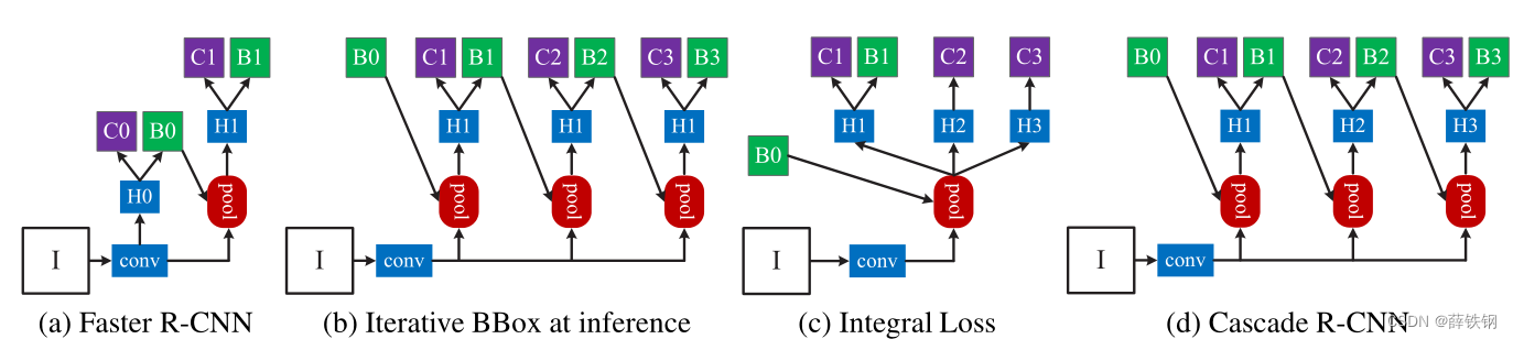
Figure 3. The architectures of different frameworks. “I” is input image, “conv” backbone convolutions, “pool” region-wise feature extraction, “H” network head, “B” bounding box, and “C” classification. “B0” is proposals in all architectures.

图3。不同框架的体系结构。“I”为输入图像，“conv”为backbone部分的卷积，“pool”为区域特征提取，“H”为网络头，“B”为边界框，“C”为分类。“B0”是所有架构中的区域建议框。

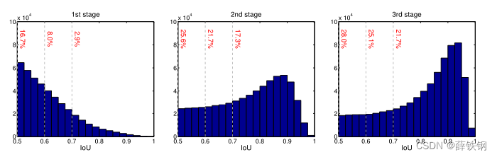
Figure 4. The IoU histogram of training samples. The distribution at 1st stage is the output of RPN. The red numbers are the positive percentage higher than the corresponding IoU threshold.

图4。训练样本的IoU直方图。第一阶段的分布是RPN的输出。红色数字是高于相应IoU阈值的正百分比。

4. Cascade R-CNN

In this section we introduce the proposed Cascade R-CNN object detection architecture of Figure 3 (d).

在本节中，我们将介绍图3 (d)所提议的Cascade R-CNN目标检测体系结构。

4.1. Cascaded Bounding Box Regression

As seen in Figure 1 ( c ), it is very difficult to ask a single regressor to perform perfectly uniformly at all quality levels. The difficult regression task can be decomposed into a sequence of simpler steps, inspired by the works of cascade pose regression [6] and face alignment [2, 32]. In the Cascade R-CNN, it is framed as a cascaded regression problem, with the architecture of Figure 3 (d). This relies on a cascade of specialized regressors
$$f(x,b)=f_{T}o{f}_{T-1}o...o{f}_1(x,b)\text{\hspace{1em}(7)}$$
where $T$ is the total number of cascade stages. Note that each regressor $f_t$ in the cascade is optimized w.r .t. the sample distribution $b^t$ arriving at the corresponding stage, instead of the initial distribution of $b^1$. This cascade improves hypotheses progressively.

如图1 ( c )所示，要求一个回归函数在所有质量水平上都能完美一致地表现是非常困难的。困难的回归任务可以分解为一系列更简单的步骤，灵感来自级联姿态回归[6]和面部对齐[2,32]。在Cascade R-CNN中，它被框定为一个级联回归问题，结构如图3 (d)所示。这依赖于专门的回归器的级联
$$f(x,b)=f_{T}o{f}_{T-1}o...o{f}_1(x,b)\text{\hspace{1em}(7)}$$
其中，T为级联的总级数。注意，级联中的每个回归器$f_t$ 都是对到达相应阶段的样本分布$b^t$的优化，而不是对初始分布$b^1$进行优化。这种级联逐步提高建议框的质量。

It differs from the iterative BBox architecture of Figure 3 (b) in several ways. First, while iterative BBox is a post-processing procedure used to improve bounding boxes, cascaded regression is a resampling procedure that changes the distribution of hypotheses to be processed by the different stages. Second, because it is used at both training and inference, there is no discrepancy between training and inference distributions. Third, the multiple specialized regressors $f_T,f_{T-1},\cdot \cdot \cdot ,f_1$ are optimized for the resampled distributions of the different stages. This opposes to the single f of (3), which is only optimal for the initial distribution. These differences enable more precise localization than iterative BBox, with no further human engineering.

它与图3 (b)的迭代BBox结构在几个方面有所不同。首先，迭代BBox是一种用于改进边界框的后处理过程，而级联回归是一种重新采样的过程，它改变了不同阶段要处理的建议框的分布。其次，因为级联回归同时用于训练和测试，所以训练和测试分布之间没有差异。第三，针对不同阶段的重采样分布，优化多个专业回归器$f_T,f_{T-1},\cdot \cdot \cdot ,f_1$。这与(3)的单一f相反，后者仅对初始分布最优。这些差异使得定位比迭代BBox更精确，不需要进一步的人工工程。

As discussed in Section 3.1, $\Delta ={\delta }_x,{\delta }_y,{\delta }_w,{\delta }_h$ in (2) needs to be normalized by its mean and variance for effective multi-task learning. After each regression stage, these statistics will evolve sequentially, as displayed in Figure 2. At training, the corresponding statistics are used to normalize $\Delta$ at each stage.

如3.1节所述，为了进行有效的多任务学习，需要对( 2 )中的$\Delta ={\delta }_x,{\delta }_y,{\delta }_w,{\delta }_h$进行均值和方差归一化。在每个回归阶段之后，这些统计量将依次演化，如图2所示。在训练时，使用相应的统计量对每个阶段的$\Delta$进行归一化处理。

4.2. Cascaded Detection

As shown in the left of Figure 4, the distribution of the initial hypotheses, e.g. RPN proposals, is heavily tilted towards low quality. This inevitably induces ineffective learning of higher quality classifiers. The Cascade R-CNN addresses the problem by relying on cascade regression as a resampling mechanism. This is is motivated by the fact that in Figure 1 © all curves are above the diagonal gray line, i.e. a bounding box regressor trained for a certain u tends to produce bounding boxes of higher IoU. Hence, starting from a set of examples $(x_i,b_i)$, cascade regression successively resamples an example distribution $(x_i^{{}^{\prime }},b_i^{{}^{\prime }})$ of higher IoU. In this manner, it is possible to keep the set of positive examples of the successive stages at a roughly constant size, even when the detector quality (IoU threshold) is increased. This is illustrated in Figure 4, where the distribution tilts more heavily towards high quality examples after each resampling step. Two consequences ensue. First, there is no overfitting, since examples are plentiful at all levels. Second, the detectors of the deeper stages are optimized for higher IoU thresholds. Note that, some outliers are sequentially removed by increasing IoU thresholds, as illustrated in Figure 2, enabling a better trained sequence of specialized detectors.

如图4左图所示，初始假设的分布如图4所示。RPN提案严重向低质量倾斜。这不可避免地会诱发更高质量分类器的无效学习。级联R - CNN依靠级联回归作为重采样机制来解决该问题。这是由于在图1 ( c )中，所有曲线都在对角线灰线的上方，即对于某个u，训练的边界框回归器倾向于产生IoU较高的边界框。因此，从一组样本$(x_i,b_i)$开始，级联回归依次对IoU较高的样本分布$(x_i^{{}^{\prime }},b_i^{{}^{\prime }})$进行重采样。通过这种方式，即使在提高检测器质量（IoU阈值）的情况下，也可以将连续阶段的正样本集保持在大致恒定的大小。这在图4中得到了说明，在每个重采样步骤之后，分布更多地向高质量的示例倾斜。随之而来的两个结果。首先，不存在过拟合现象，因为各个层次的例子都很丰富。其次，更深阶段的检测器针对更高的IoU阈值进行了优化。值得注意的是，通过增加IoU阈值，一些异常值被依次移除，如图2所示，从而实现训练有素的专用检测器序列。

At each stage $t$, the R-CNN includes a classifier $h_t$ and a regressor $f_t$ optimized for IoU threshold $u_t$, where $u^t>u^{t-1}$. This is guaranteed by minimizing the loss
$$L(x^t,g)=L_{cls}(h_t(x^t),y^t)+\lambda [y^t\ge 1]L_{loc}(f_t(x^t,b^t),g)\text{\hspace{1em}(8)}$$
where $b^t=f_{t-1}(x^{t-1},b^{t-1})$,$g$ is the ground truth object for $x_t$, $\lambda =1$ the trade-off coefficient, [·] the indicator function, and $y_t$ is the label of $x_t$ given $u_t$ by (5). Unlike the integral loss of (6), this guarantees a sequence of effectively trained detectors of increasing quality. At inference, the quality of the hypotheses is sequentially improved, by applications of the same cascade procedure, and higher quality detectors are only required to operate on higher quality hypotheses. This enables high quality object detection, as suggested by Figure 1 © and (d).

在每个阶段$t$，R - CNN包括一个分类器$h_t$和一个针对IoU阈值$u_t$优化的回归器$f_t$，其中$u^t>u^{t-1}$。这是通过最小化损失来保证的
$$L(x^t,g)=L_{cls}(h_t(x^t),y^t)+\lambda [y^t\ge 1]L_{loc}(f_t(x^t,b^t),g)\text{\hspace{1em}(8)}$$
其中，$b^t=f_{t-1}(x^{t-1},b^{t-1})$，g是$x_t$的ground truth对象，$\lambda =1$是权衡系数，[ · ]是指示函数，$y_t$是$u_t$由式( 5 )给出的$x_t$的标签。与( 6 )式的积分损失不同，这保证了一系列有效训练的检测器质量不断提高。在测试时，通过应用相同的级联过程，建议框的质量被依次提高，并且更高质量的检测器只需要对更高质量的建议框进行操作。如图1 ( c )和( d )所示，这可以实现高质量的目标检测。

5. Experimental Results

The Cascade R-CNN was evaluated on MS-COCO 2017 [20], which contains ∼118k images for training, 5k for validation (val) and ∼20k for testing without provided annotations (test-dev). The COCO-style Average Precision (AP) averages AP across IoU thresholds from 0.5 to 0.95 with an interval of 0.05. These evaluation metrics measure the detection performance of various qualities. All models were trained on COCO training set, and evaluated on val set. Final results were also reported on test-dev set.

在MS-COCO 2017[20]上评估Cascade R-CNN，其中包含用于训练的118k张图像，用于验证( val )的5k张图像和用于测试的20k图像（不含标签test-dev）。COCO-style Average Precision ( AP )在IoU阈值范围内的平均AP为0.5 ~ 0.95，间隔为0.05。这些评价指标衡量各种质量的检测性能。所有模型均在COCO训练集上进行训练，并在val训练集上进行评价。最后的结果也在test - dev集上报告。

5.1. Implementation Details

All regressors are class agnostic for simplicity. All cascade detection stages in Cascade R-CNN have the same architecture, which is the head of the baseline detection network. In total, Cascade R-CNN have four stages, one RPN and three for detection with $U=0.5,0.6,0.7$, unless otherwise noted. The sampling of the first detection stage follows [11, 27]. In the following stages, resampling is implemented by simply using the regressed outputs from the previous stage, as in Section 4.2. No data augmentation was used except standard horizontal image flipping. Inference was performed on a single image scale, with no further bells and whistles. All baseline detectors were reimplemented with Caffe [18], on the same codebase for fair comparison.

为了简单起见，所有回归器都是类不可知的。Cascade R-CNN中的所有级联检测阶段具有相同的架构，是基线检测网络的头部。Cascade R-CNN总共有4个阶段，1个RPN和3个检测器，检测器的U取值为：$U=0.5,0.6,0.7$，除非另有说明。第一个检测阶段的采样遵循[11、27]。在接下来的阶段中，通过简单地使用前一阶段的回归输出来实现重新采样，如4.2节所述。除标准水平图像翻转外，未使用数据增强。测试是在单个图像尺度上进行的，没有其他花里胡哨的深度神经网络的技巧（任何人都可以不通各种精调，各种扩大训练集，各种hard online就可以达到比较好的效果）。所有基线检测器均使用Caffe [18]重新实现，在同一代码库上进行公平比较。

5.1.1 Baseline Networks

To test the versatility of the Cascade R-CNN, experiments were performed with three popular baseline detectors: Faster-RCNN with backbone VGG-Net [29], R-FCN [4] and FPN [21] with ResNet backbone [16]. These baselines have a wide range of detection performances. Unless noted, their default settings were used. End-to-end training was used instead of multi-step training.

为了测试Cascade R-CNN的多功能性，使用三种常用的基线检测器进行了实验：基于VGG-Net[29]的Faster-RCNN，基于ResNet[16]的R-FCN[4]和FPN[21]。这些基线具有广泛的检测性能。除非特别说明，否则使用默认设置。采用端到端训练代替多步训练。

Faster-RCNN: The network head has two fully connected layers. To reduce parameters, we used [13] to prune less important connections. 2048 units were retained per fully connected layer and dropout layers were removed. Training started with a learning rate of 0.002, reduced by a factor of 10 at 60k and 90k iterations, and stopped at 100k iterations, on 2 synchronized GPUs, each holding 4 images per iteration. 128 RoIs were used per image.

Faster-RCNN: 网络头有两个全连接层。为了减少参数，我们使用[13]来去掉不太重要的连接。每个全连接层保留2048个单元，去掉dropout层。训练开始时学习率为0.002，在60k和90k迭代时降低10倍，在100k迭代时停止，在2个同步gpu上，每个gpu每次迭代保存4张图像。每张图像使用128个RoIs。

R-FCN: R-FCN adds a convolutional, a bounding box regression, and a classification layer to the ResNet. All heads of the Cascade R-CNN have this structure. Online hard negative mining [28] was not used. Training started with a learning rate of 0.003, which was decreased by a factor of 10 at 160k and 240k iterations, and stopped at 280k iterations, on 4 synchronized GPUs, each holding one image per iteration. 256 RoIs were used per image.

R-FCN: R-FCN为ResNet增加了卷积、边界框回归层和分类层。Cascade R-CNN的所有头部都有这个结构。未采用困难负样本（即假阳性）挖掘[28]。训练开始时学习率为0.003，在160k和240k迭代时下降10倍，并在280k迭代时停止，在4个同步gpu上，每个gpu每次迭代保存一张图像。每张图像使用256个RoIs。

FPN: Since no source code is publicly available yet for FPN, our implementation details could be different. RoIAlign [14] was used for a stronger baseline. This is denoted as FPN+ and was used in all ablation studies. As usual, ResNet-50 was used for ablation studies, and ResNet-101 for final detection. Training used a learning rate of 0.005 for 120k iterations and 0.0005 for the next 60k iterations, on 8 synchronized GPUs, each holding one image per iteration. 256 RoIs were used per image.

FPN: 由于FPN还没有公开的源代码，我们的实现细节可能有所不同。RoIAlign[14]用于更强的基线。这被记为FPN+，用于所有的消融研究。通常，ResNet-50用于消融研究，ResNet-101用于最终检测。在8个同步GPU上，每次迭代保持一幅图像，训练在120k次迭代中使用0.005的学习率，在接下来的60k次迭代中使用0.0005的学习率。每幅图像使用256个RoIs。

5.2. Quality Mismatch

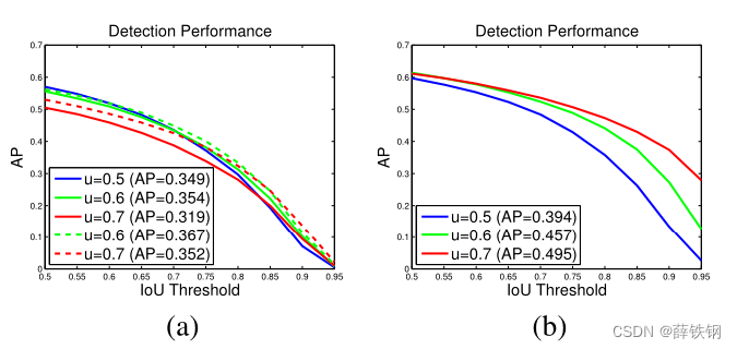
Figure 5. (a) is detection performance of individually trained detectors, with their own proposals (solid curves) or Cascade R-CNN
stage proposals (dashed curves), and (b) is by adding ground truth to the proposal set.

图5。(a)是单独训练的检测器的检测性能，具有自己的建议(实线曲线)或Cascade R-CNN阶段建议(虚线曲线)，(b)是将真实边界框添加到候选集时得到的结果。

Figure 5 (a) shows the AP curves of three individually trained detectors of increasing IoU thresholds of $U=0.5,0.6,0.7$. The detector of $u=0.5$ outperforms the detector of $u=0.6$ at low IoU levels, but underperforms it at higher levels. However, the detector of $u=0.7$ underperforms the other two. To understand why this happens, we changed the quality of the proposals at inference. Figure 5 (b) shows the results obtained when ground truth bounding boxes were added to the set of proposals. While all detectors improve, the detector of u = 0.7 has the largest gains, achieving the best performance at almost all IoU levels. These results suggest two conclusions. First, $u=0.5$ is not a good choice for precise detection, simply more robust to low quality proposals. Second, highly precise detection requires hypotheses that match the detector quality. Next, the original detector proposals were replaced by the Cascade R-CNN proposals of higher quality ($u=0.6$ and $u=0.7$ used the 2nd and 3rd stage proposals, respectively). Figure 5 (a) also suggests that the performance of the two detectors is significantly improved when the testing proposals closer match the detector quality.

图5 ( a )展示了三个单独训练的检测器在提高$U=0.5,0.6,0.7$的IoU阈值时的AP曲线。$u=0.5$检测器在低IoU水平下优于$u=0.6$检测器，但在高IoU水平下表现较差。但$u=0.7$的探测器性能逊于其他两种。为了理解为什么会出现这种情况，我们在测试时改变了建议框的质量。图5 ( b )展示了将真实边界框添加到候选集时得到的结果。在所有检测器改进的同时，$u=0.7$的检测器具有最大的增益，在几乎所有的IoU水平上都取得了最好的性能。这些结果提示了两个结论。首先，$u=0.5$对于精确检测不是一个好的选择，对于低质量的提议更鲁棒。其次，高精度的检测需要与检测器质量相匹配的建议框。接下来，将原来的检测器建议替换为质量更高的( $u=0.6$和$u=0.7$分别采用第2阶段和第3阶段方案)的Cascade R-CNN提案。图5 ( a )也表明，当测试方案与检测器质量更加匹配时，两种检测器的性能都有明显的提升。

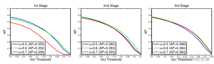
Figure 6. The detection performance of all Cascade R-CNN detectors at all cascade stages.

图6。所有Cascade R-CNN检测器在所有级联阶段的检测性能。

Testing all Cascade R-CNN detectors at all cascade stages produced similar observations. Figure 6 shows that each detector was improved when used more precise hypotheses, while higher quality detector had larger gain. For example, the detector of $u=0.7$ performed poorly for the low quality proposals of the 1st stage, but much better for the more precise hypotheses available at the deeper cascade stages. In addition, the jointly trained detectors of Figure 6 outperformed the individually trained detectors of Figure 5 (a), even when the same proposals were used. This indicates that the detectors are better trained within the Cascade R-CNN framework.

在所有级联阶段测试所有Cascade R-CNN检测器产生了类似的观测结果。从图6可以看出，当使用更精确的建议框时，每个检测器都得到了改善，而更高质量的检测器具有更大的增益。例如，$u=0.7$的检测器对于第一阶段的低质量建议表现较差，但对于更深层的级联阶段可用的更精确的建议框表现更好。此外，即使采用相同的方案，图6的联合训练检测器也优于图5 ( a )的单独训练检测器。这表明在Cascade R-CNN框架下，检测器得到了更好的训练。

5.3. Comparison with Iterative BBox and Integral Loss

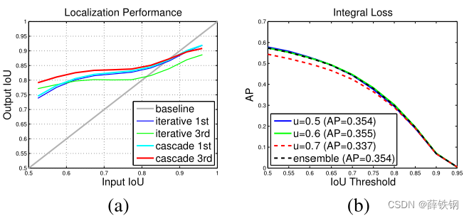
Figure 7. (a) is the localization comparison, and (b) is the detection performance of individual classifiers in the integral loss detector.

图7。(a)为局部化比较，(b)为单个分类器在积分损耗检测器中的检测性能。

In this section, we compare the Cascade R-CNN to iterative BBox and the integral loss detector. Iterative BBox was implemented by applying the FPN+ baseline iteratively, three times. The integral loss detector has the same number of classification heads as the Cascade R-CNN, with $U=0.5,0.6,0.7.$

在本节中，我们将Cascade R-CNN与迭代BBox和积分损失检测器进行比较。迭代BBox通过迭代应用FPN +基线实现，共3次。积分损失检测器具有与Cascade R-CNN相同数量的分类头，$U=0.5,0.6,0.7$

Localization: The localization performances of cascade regression and iterative BBox are compared in Figure 7 (a). The use of a single regressor degrades localization for hypotheses of high IoU. This effect accumulates when the regressor is applied iteratively, as in iterative BBox, and performance actually drops. Note the very poor performance of iterative BBox after 3 iterations. On the contrary, the cascade regressor has better performance at later stages, out-performing iterative BBox at almost all IoU levels.

定位： 图7 ( a )对比了级联回归和迭代BBox的定位性能。使用单个回归器降低了高IoU建议框的局部化。这种影响在迭代应用回归器时累积，如迭代BBox时，性能实际上下降了。注意到迭代BBox在迭代3次后性能很差。相反，级联回归器在后期具有更好的性能，在几乎所有的IoU级别上都优于迭代BBox。

Integral Loss: The detection performances of all classifiers in the integral loss detector, sharing a single regressor, are shown in Figure 7 (b). The classifier of $u=0.6$ is the best at all IoU levels, while the classifier of $u=0.7$ is the worst. The ensemble of all classifiers shows no visible gain.

积分损失： 积分损失检测器中各分类器共享一个回归器的检测性能如图7 (b)所示，在所有IoU级别上，$u=0.6$的分类器的检测性能最好，$u=0.7$的分类器的检测性能最差。所有分类器的集合没有显示出明显的增益。

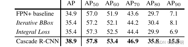
Table 1. The comparison with iterative BBox and integral loss.

表1。与迭代BBox和积分损失的比较。

Table 1 shows, both iterative BBox and integral loss detector improve the baseline detector marginally. The cascade R-CNN has the best performance for all evaluation metrics. The gains are mild for low IoU thresholds but significant for the higher ones.

从表1可以看出，迭代BBox和积分损失检测器对基线检测器都有一定的改善。cascade R-CNN在所有评估指标中具有最佳性能。对于较低的IoU阈值，提升是不显著的，但对于较高的IoU阈值，提升是显著的。

5.4. Ablation Experiments

Ablation experiments were also performed.

接下来进行了消融实验。

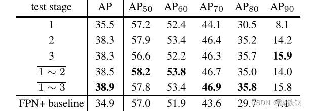
Table 2. The stage performance of Cascade R-CNN. 1 ∼ 3 indicates the ensemble of three classifiers on the 3rd stage proposals.

表2。Cascade R-CNN的阶段表现。1 ~ 3表示第三阶段提案中三个分类器的集合。

Stage-wise Comparison: Table 2 summarizes stage performance. The 1st stage already outperforms the baseline detector, due to the benefits of multi-stage multi-task learning. The 2nd stage improves performance substantially, and the 3rd is equivalent to the 2nd. This differs from the integral loss detector, where the higher IOU classifier is relatively weak. While the former (later) stage is better at low (high) IoU metrics, the ensemble of all classifiers is the best overall.

不同阶段之间的比较： 表2总结了阶段表现。由于多阶段多任务学习的好处，第一阶段已经优于基线检测器。第二阶段性能大幅提升，第三阶段与第二阶段相当。这与积分损失检测器不同，在积分损失检测器中，较高的IOU分类器相对较弱。虽然前(后)阶段在低(高)IoU指标上表现更好，但所有分类器的集成总体上是最好的。

IoU Thresholds: A preliminary Cascade R-CNN was trained using the same IoU threshold $u=0.5$ for all heads. In this case, the stages differ only in the hypotheses they receive. Each stage is trained with the corresponding hypotheses, i.e. accounting for the distributions of Figure 2.The first row of Table 3 shows that the cascade improves on the baseline detector. This suggests the importance of optimizing stages for the corresponding sample distributions. The second row shows that, by increasing the stage threshold $u$, the detector can be made more selective against close false positives and specialized for more precise hypotheses, leading to additional gains. This supports the conclusions of Section 4.2.

IoU阈值： 对所有头部使用相同的IoU阈值$u=0.5$训练一个初步的Cascade R-CNN。在这种情况下，各阶段仅在所接受的建议框上存在差异。每个阶段都使用相应的建议框进行训练，即考虑图2的分布。表3的第一行显示了级联在基线检测器上的改进。这表明优化阶段对于相应样本分布的重要性。第二行显示，通过增加阶段阈值$u$，可以使检测器对“接近假阳性”具有更高的选择性，并专注于更精确的建议框，从而获得额外的增益。这支持了4.2节的结论。

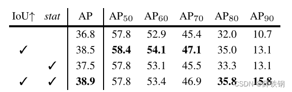
Table 3. The ablation experiments. “IoU↑” means increasing IoU thresholds, and “stat” exploiting sequential regression statistics.

表3。消融实验。“IoU↑”表示增加IoU阈值，“stat”利用顺序回归统计。

Regression Statistics: Exploiting the progressively updated regression statistics, of Figure 2, helps the effective multi-task learning of classification and regression. Its benefit is noted by comparing the models with/without it in Table 3. The learning is not sensitive to these statistics.

回归统计： 利用图2中逐步更新的回归统计信息，有助于有效地进行分类和回归的多任务学习。通过比较表3中有/没有它的模型，可以看出它的优势。学习对这些统计数据不敏感。

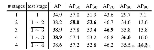
Table 4. The impact of the number of stages in Cascade R-CNN.

表4。Cascade R-CNN中阶段数量的影响。

Number of Stages: The impact of the number of stages is summarized in Table 4. Adding a second detection stage significantly improves the baseline detector. Three detection stages still produce non-trivial improvement, but the addition of a 4th stage ($u=0.75$) led to a slight performance decrease. Note, however, that while the overall AP performance degrades, the four-stage cascade has the best performance for high IoU levels. The three-stage cascade achieves the best trade-off.

阶段数量： 阶段数量的影响如表4所示。添加第二个检测阶段显著改善了基线检测器。三个检测阶段仍然产生了不小的改进，但添加第四个阶段（$u=0.75$）导致性能略有下降。但是，请注意，虽然总体AP性能下降，但对于高IoU级别，四级级联具有最佳性能。三级级联实现了最佳的权衡。

5.5. Comparison with the state-of-the-art

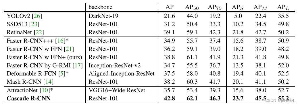
Table 5. Comparison with the state-of-the-art single-model detectors on COCO test-dev. The entries denoted by “*” used bells and whistles at inference.

表5。与COCO测试开发中最先进的单模型探测器的比较。用“*”表示的条目在测试时使用了深度神经网络的其他技巧以获得最佳效果。

The Cascade R-CNN, based on FPN+ and ResNet-101 backbone, is compared to state-of-the-art single-model object detectors in Table 5. The settings are as described in Section 5.1.1, but a total of 280k training iterations were run and the learning rate dropped at 160k and 240k iterations. The number of RoIs was also increased to 512. The first group of detectors on Table 5 are one-stage detectors, the second group two-stage, and the last group multi-stage (3-stages+RPN for the Cascade R-CNN). All the compared state-of-the-art detectors were trained with $u=0.5$. It is noted that our FPN+ implementation is better than the original FPN [21], providing a very strong baseline. In addition, the extension from FPN+ to Cascade R-CNN improved performance by ∼4 points. The Cascade R-CNN also outperformed all single-model detectors by a large margin, under all evaluation metrics. This includes the single-model entries of the COCO challenge winners in 2015 and 2016 (Faster R-CNN+++ [16], and G-RMI [17]), and the very recent Deformable R-FCN [5], RetinaNet [22] and Mask R-CNN [14]. The best multi-stage detector on COCO, AttractioNet [10], used iterative BBox for proposal generation. Although many enhancements were used in AttractioNet, the vanilla Cascade R-CNN still outperforms it by 7.1 points. Note that, unlike Mask R-CNN, no segmentation information is exploited in the Cascade R-CNN. Finally, the vanilla single-model Cascade R-CNN also surpasses the heavily engineered ensemble detectors that won the COCO challenge in 2015 and 2016 (AP 37.4 and 41.6, respectively).

基于FPN+和ResNet-101主干的Cascade R-CNN与最先进的单模型目标检测器进行了比较，见表5。设置如5.1.1节所述，但是总共运行了280k次训练迭代，在160k和240k次迭代时学习率下降。RoIs的数量也增加到512个。表5中的第一组检测器为单级检测器，第二组为两级检测器，最后一组为多级检测器（Cascade R-CNN为3级+RPN）。所有比较先进的检测器都被训练为$u=0.5$。值得注意的是，我们的FPN+实现比原来的FPN[21]更好，提供了一个非常强的基线。此外，从FPN+扩展到Cascade R-CNN，性能提高了约4点。在所有评估指标下，Cascade R-CNN的表现也超过了所有单模型检测器。这包括2015年和2016年COCO挑战赛冠军的单模型参赛作品（Faster R-CNN+++[16]和G-RMI[17]），以及最近的变形R-FCN [5]， RetinaNet[22]和Mask R-CNN[14]。COCO上最好的多级检测器AttractioNet[10]使用迭代BBox来生成提案。尽管在AttractioNet中使用了许多增强功能，但香草（vanilla）模型 Cascade R-CNN的表现仍然超过了它7.1分。请注意，与Mask R-CNN不同，Cascade R-CNN中没有利用分割信息。最后，香草（vanilla）模型Cascade R-CNN也超过了2015年和2016年赢得COCO挑战的精心设计的集成检测器(AP 37.4和41.6)1。

5.6. Generalization Capacity

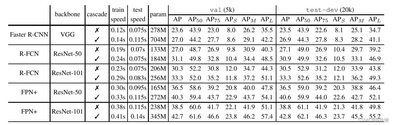
Table 6. Detailed comparison on multiple popular baseline object detectors. All speeds are reported per image on a single Titan Xp GPU.

表6。详细比较了多种流行的基线对象检测器。在单个Titan Xp GPU上报告每个图像的所有速度。

Three-stage Cascade R-CNN of all three baseline detectors are compared in Table 6. All settings are as above, with the changes of Section 5.5 for FPN+.

表6比较了三种基线检测器的三级Cascade R-CNN。所有设置如上所述，FPN+的变化如5.5节。

Detection Performance: Again, our implementations are better than the original detectors [27, 4, 21]. Still, the Cascade R-CNN improves on these baselines consistently by 2∼4 points, independently of their strength. These gains are also consistent on val and test-dev. These results suggest that the Cascade R-CNN is widely applicable across detector architectures.

检测性能： 同样，我们的实现比原来的检测器更好[27,4,21]。尽管如此，Cascade R-CNN在这些基线上持续提高2 ~ 4个点，与它们的强度无关。这些提升效果在验证集val和测试集test-dev上也是一致的。这些结果表明Cascade R-CNN广泛适用于检测器架构。

Parameter and Timing: The number of the Cascade R-CNN parameters increases with the number of cascade stages. The increase is linear in the parameter number of the baseline detector heads. In addition, because the computational cost of a detection head is usually small when compared to the RPN, the computational overhead of the Cascade R-CNN is small, at both training and testing.

参数和时间： Cascade RCNN参数的数量随着级联级数的增加而增加。基线探测器头的参数数量呈线性增加。此外，由于与RPN相比，检测头的计算成本通常很小，Cascade R-CNN的计算开销在训练和测试中都很小。

6. Conclusion

In this paper, we proposed a multi-stage object detection framework, the Cascade R-CNN, for the design of high quality object detectors. This architecture was shown to avoid the problems of overfitting at training and quality mismatch at inference. The solid and consistent detection improvements of the Cascade R-CNN on the challenging COCO dataset suggest the modeling and understanding of various concurring factors are required to advance object detection. The Cascade R-CNN was shown to be applicable to many object detection architectures. We believe that it can be useful to many future object detection research efforts.

在本文中，我们提出了一个多级目标检测框架，Cascade R-CNN，用于设计高质量的目标检测器。这种架构被证明可以避免训练时的过拟合和测试时的质量不匹配问题。Cascade R-CNN在具有挑战性的COCO数据集上的可靠和一致的检测改进表明，需要对各种并发因素进行建模和理解，以推进目标检测。Cascade R-CNN被证明适用于许多目标检测架构。我们相信它对未来的许多目标检测研究工作是有用的。