


每天给你送来NLP技术干货!
编辑:AI算法小喵
写在前面
在《一文详解生成式文本摘要经典论文Pointer-Generator》中,我们已经详细地介绍过长文本摘要模型 PGN+Coverage。这个工作小喵20年初的时候不仅研读了,同时也做了相关的复现与优化尝试,没记错的话当时用的是TF框架。碍于年代久远,当时也没有做笔记的习惯,所以没法跟大家分享相关的实践内容。
不过,小喵最近发现了一篇与之相关实践类博文,作者将 PGN+Coverage 用在营销文本生成任务上。整个实验与代码实现写的非常详细,里面不仅设计模型本身,还包含生成任务的评估方法、深度学习训练的优化技巧、文本增强技术等内容。好东西当然不能藏着掖着了,这不小喵赶在中秋节这天来跟大家分享了,让我们一起学习讨论,共同进步吧!
鉴于本文比较长,内容较多,建议大家收藏码住,后面再细看!另外,祝大家中秋快乐,好好过节呀!月饼好好吃啊,这些天我已经吃了很多种口味的月饼了,比如今天就吃了广式纯正五仁月饼、滇式老云腿月饼。不过月饼比较重口味,家里矿泉水又刚好喝完了,吃完月饼嘴巴特别干,这会儿正喝着牛奶解渴😂。
0. 引言
文本生成(Text Generation)可进一步细分为文本摘要、机器翻译、故事续写等任务。本项目主要用到文本摘要技术。
抽取式摘要是选取其中关键的句子摘抄下来。相反,生成式摘要则是希望通过学习原文的语义信息后相应地生成一段较短但是能反映其核心思想的文本作为摘要。
生成式摘要相较于抽取式摘要更加灵活,但也更加难以实现。在本项目中,我们将先用生成式摘要的方法构建 Seq2seq+Attention 的模型作为 Baseline,然后构建一个结合生成式和抽取式两种方法的 Pointer-Generator Network(PGN)模型。
通过本项目中,可以学习到:
熟练掌握(
Seq2seq、Attention、LSTM、PGN 、converage等模型)的实现。熟练掌握如何训练神经网络(
调参、debug、可视化)。熟练掌握如何实现
Beam Search算法来生成文本。熟练掌握文本生成任务的
评估方法。掌握深度学习训练的一些优化技巧,如:
Scheduled sampling、Weight tying等)。了解如何使用多种
文本增强技术处理少样本问题。
1. 项目任务简介
文本生成任务中,通常将作为输入的原文称为 source,将待生成的目标文本称为 target 或者 hypothesis,将用来作为 target 好坏的参考文本称之为reference。
本项目的数据来自「京东电商的发现好货栏目」,其中source 主
要由三部分构成:
商品的标题;
商品的参数;
商品宣传图片里提取出来的宣传文案(借助OCR技术提取)。
参考文本如下图所示:

商品标题:

商品参数:
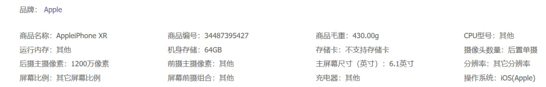
商品宣传图片:

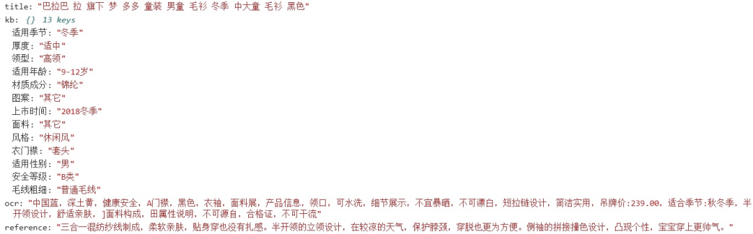
1. 数据预处理
首先数据格式如下图所示,为一个json文件,里面的title、kb以及ocr是我们利用的source,reference可以看作我们的标签。
1.1 将json文件转化成txt文件
就是一个读取json,写入txt的文件,不再赘述。
json_path = os.path.join(abs_path, '服饰_50k.json')
with open(json_path, 'r', encoding='utf8') as file:
    jsf = json.load(file)
for jsobj in jsf.values():
    title = jsobj['title'] + ' '  # Get title.
    kb = dict(jsobj['kb']).items()  # Get attributes.
    kb_merged = ''
    for key, val in kb:
        kb_merged += key+' '+val+' '  # Merge attributes.
    ocr = ' '.join(list(jieba.cut(jsobj['ocr'])))  # Get OCR text.
    texts = []
    texts.append(title + ocr + kb_merged)  # Merge them.
    reference = ' '.join(list(jieba.cut(jsobj['reference'])))
    for text in texts:
        sample = text+'<sep>'+reference  # Seperate source and reference.
        samples.add(sample)
write_path = os.path.join(abs_path, '../files/samples.txt')
write_samples(samples, write_path)
1.2 词典处理
add_words函数:向词典⾥加⼊⼀个新词,需要完成对word2index、index2word和word2count三个变量的更新。
class Vocab(object):
    def __init__(self):
        self.word2index = {}
        self.word2count = Counter()
        self.reserved = ['<PAD>', '<SOS>', '<EOS>', '<UNK>']
        self.index2word = self.reserved[:]
        self.embeddings = None
    def add_words(self, words):
        """Add a new token to the vocab and do mapping between word and index.
        """
        for word in words:
            if word not in self.word2index:
                self.word2index[word] = len(self.index2word)
                self.index2word.append(word)
self.word2count.update(words)build_vocab函数:需要实现控制数据集词典的⼤⼩(从config.max_vocab_size)读取这⼀参数。我们这里使⽤ python 的 collection 模块中的 Counter 来做。
def build_vocab(self, embed_file: str = None) -> Vocab:
        """Build the vocabulary for the data set.
        """
        # word frequency
        word_counts = Counter()
        count_words(word_counts, [src + tgr for src, tgr in self.pairs])
        vocab = Vocab()
        # Filter the vocabulary by keeping only the top k tokens in terms of
        # word frequncy in the data set
        for word, count in word_counts.most_common(config.max_vocab_size):
            vocab.add_words([word])
        if embed_file is not None:
            count = vocab.load_embeddings(embed_file)
            print("%d pre-trained embeddings loaded." % count)
        return vocab


def count_words(counter, text):
    '''Count the number of occurrences of each word in a set of text'''
    for sentence in text:
        for word in sentence:
            counter[word] += 1
1.3 自定义数据集SampleDataset(Dataset类)
我们知道用 dataset 和 dataloader 来进行数据加载读取和训练方便,这里我们自定义了SampleDataset。如下所示,其中我们要具体讲一讲__getitem__函数。
class SampleDataset(Dataset):
    """The class represents a sample set for training.
    """
    def __init__(self, data_pair, vocab):
        self.src_sents = [x[0] for x in data_pair]
        self.trg_sents = [x[1] for x in data_pair]
        self.vocab = vocab
        self._len = len(data_pair)
    def __getitem__(self, index):
        x, oov = source2ids(self.src_sents[index], self.vocab)
        return {
            'x': [self.vocab.SOS] + x + [self.vocab.EOS],
            'OOV': oov,
            'len_OOV': len(oov),
            'y': [self.vocab.SOS] +
            abstract2ids(self.trg_sents[index],
                         self.vocab, oov) + [self.vocab.EOS],
            'x_len': len(self.src_sents[index]),
            'y_len': len(self.trg_sents[index])
        }
    def __len__(self):
return self._len__getitem__函数通用目的是获取第index个数据。具体在我们的项目中,我们想要利用 __getitem__获取第index个文本数据的ids。
source 文本
在 __getitem__ 中,我们所调用的 source2ids不仅完成了source文本中的 token 到 id 的映射,同时也处理了source文本中的 OOV 的 token。
具体来说,对于source文本中的OOV token(即不在既定词表中的词),我们将其映射到词表的最末尾并编号表示。换句话说,若我们的词表大小为5000,则 OOV token 会依次被编号为5001、5002、5003...。
def source2ids(source_words, vocab):
    ids = []
    oovs = []
    unk_id = vocab.UNK
    for w in source_words:
        i = vocab[w]
        if i == unk_id:
            if w not in oovs:
                oovs.append(w)
            # This is 0 for the first source OOV, 1 for the second source OOV
            oov_num = oovs.index(w)
            # This is e.g. 20000 for the first source OOV, 50001 for the second
            ids.append(vocab.size() + oov_num)
        else:
            ids.append(i)
    return ids, oovs
reference 文本
对于reference文本,我们利用 abstract2ids 函数将 reference 文本映射成ids。需要注意的是,PGN可以⽣成在source⾥⾯出现过的OOV tokens,所以我们对reference的token的映射方式将不同于以往(以往通常将reference中的OOV toekn直接替换为“”)。
具体地,我们需要将在source 文本中出现过的OOV tokens也记录下来并给它们相应的临时id,⽽不是直接替换为“”,这样可以使训练时的损失计算更加准确。
def abstract2ids(abstract_words, vocab, source_oovs):
    """Map tokens in the abstract (reference) to ids.
       OOV tokens in the source will be remained.
    """
    ids = []
    unk_id = vocab.UNK
    for w in abstract_words:
        i = vocab[w]
        if i == unk_id:  # If w is an OOV word
            if w in source_oovs:  # If w is an in-source OOV
                # Map to its temporary source OOV number
                vocab_idx = vocab.size() + source_oovs.index(w)
                ids.append(vocab_idx)
            else:  # If w is an out-of-source OOV
                ids.append(unk_id)  # Map to the UNK token id
        else:
            ids.append(i)
    return ids
1.4 生成Dataloader进行训练
Dataloader可以更方便的在数据集中取batch进行批训练,其中最重要的是collate_fn函数,其作用是将数据集拆分为多个批,并分别对每个批进行填充至其最大长度。
train_data = SampleDataset(dataset.pairs, v)
val_data = SampleDataset(val_dataset.pairs, v)
train_dataloader = DataLoader(dataset=train_data,
                                  batch_size=config.batch_size,
                                  shuffle=True,
                                  collate_fn=collate_fn)

def collate_fn(batch):
    """Split data set into batches and do padding for each batch.
    """
    def padding(indice, max_length, pad_idx=0):
        pad_indice = [item + [pad_idx] * max(0, max_length - len(item)) for item in indice]
        return torch.tensor(pad_indice)
    data_batch = sort_batch_by_len(batch)
    x = data_batch["x"]
    x_max_length = max([len(t) for t in x])
    y = data_batch["y"]
    y_max_length = max([len(t) for t in y])
    OOV = data_batch["OOV"]
    len_OOV = torch.tensor(data_batch["len_OOV"])
    x_padded = padding(x, x_max_length)
    y_padded = padding(y, y_max_length)
    x_len = torch.tensor(data_batch["x_len"])
    y_len = torch.tensor(data_batch["y_len"])
    return x_padded, y_padded, x_len, y_len, OOV, len_OOV
2. Baseline模型实现:seq2seq+Attention
下图是基线模型的框架如:
首先,Source 文本中的toke将被逐个送入编码器(这里为单层双向LSTM),产生一系列编码器隐藏状态 ;
然后在每个解码步骤 中,解码器(这里为单层单向LSTM)接收前一个单词的单词嵌入(在训练时,这是参考摘要的前一个单词;在测试时,它是解码器预测的前一个单词),并且具有解码器状态 。
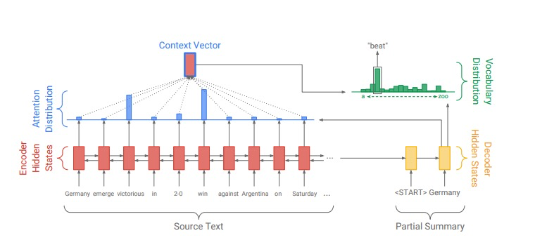
注意分布 的计算如Bahdanau等人所述: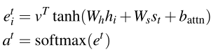
加权求和生成内容向量: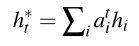
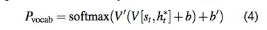
解码端得到单词分布: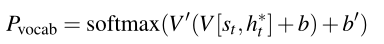
2.1 基于双向LSTM的Encoder
class Encoder(nn.Module):
    def __init__(self,vocab_size, embed_size, hidden_size, rnn_drop: float = 0):
        super(Encoder, self).__init__()
        self.embedding = nn.Embedding(vocab_size, embed_size)
        self.hidden_size = hidden_size
        self.lstm = nn.LSTM(embed_size,
                            hidden_size,
                            bidirectional=True,
                            dropout=rnn_drop,
                            batch_first=True)
    def forward(self, x):
        """Define forward propagation for the endoer.
        """
        embedded = self.embedding(x)
        output, hidden = self.lstm(embedded)
        return output, hidden
2.2 Attention及Context Vector
这个部分主要进行Attention与Context Vector的计算,具体过程如下:
处理decoder的隐状态 和 ,将⼆者拼接得到 ,并处理成合理的shape。
参考论⽂中的公式(1)和(2),实现attention weights的计算。
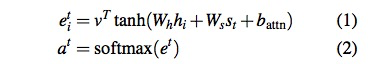
由于训练过程中会对batch中的样本进⾏padding,对于进⾏了padding的输⼊我们需要把填充的位置的attention weights给过滤掉(padding mask),然后对剩下位置的attention weights进⾏归⼀化。
根据论⽂中的公式(3)计算context vector(加权求和):
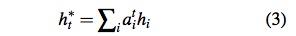
代码实现如下:
class Attention(nn.Module):
    def __init__(self, hidden_units):
        super(Attention, self).__init__()
        # Define feed-forward layers.
        self.Wh = nn.Linear(2*hidden_units, 2*hidden_units, bias=False)
        self.Ws = nn.Linear(2*hidden_units, 2*hidden_units)

    def forward(self,
                decoder_states,
                encoder_output,
                x_padding_masks,
                coverage_vector):
        """Define forward propagation for the attention network.
        """
        # Concatenate h and c to get s_t and expand the dim of s_t.
        h_dec, c_dec = decoder_states
        s_t = torch.cat([h_dec, c_dec], dim=2)
        s_t = s_t.transpose(0, 1)
        s_t = s_t.expand_as(encoder_output).contiguous()
        # calculate attention scores
        encoder_features = self.Wh(encoder_output.contiguous())
        decoder_features = self.Ws(s_t)
        att_inputs = encoder_features + decoder_features
        score = self.v(torch.tanh(att_inputs))
        attention_weights = F.softmax(score, dim=1).squeeze(2)
        attention_weights = attention_weights * x_padding_masks
        # Normalize attention weights after excluding padded positions.
        normalization_factor = attention_weights.sum(1, keepdim=True)
        attention_weights = attention_weights / normalization_factor
        context_vector = torch.bmm(attention_weights.unsqueeze(1),
                                   encoder_output)
        context_vector = context_vector.squeeze(1)
        return context_vector, attention_weights
2.3 基于单向LSTM与两个线性层的Decoder
解码端的前向传播如下:
class Decoder(nn.Module):
    def __init__(self, vocab_size, embed_size, hidden_size, enc_hidden_size=None, is_cuda=True):
        super(Decoder, self).__init__()
        self.embedding = nn.Embedding(vocab_size, embed_size)
        self.DEVICE = torch.device('cuda') if is_cuda else torch.device('cpu')
        self.vocab_size = vocab_size
        self.hidden_size = hidden_size
        self.lstm = nn.LSTM(embed_size, hidden_size, batch_first=True)
        self.W1 = nn.Linear(self.hidden_size * 3, self.hidden_size)
        self.W2 = nn.Linear(self.hidden_size, vocab_size)

    def forward(self, x_t, decoder_states, context_vector):
        """Define forward propagation for the decoder.
        """
        decoder_emb = self.embedding(x_t)
        decoder_output, decoder_states = self.lstm(decoder_emb, decoder_states)
        # concatenate context vector and decoder state
        decoder_output = decoder_output.view(-1, config.hidden_size)
        concat_vector = torch.cat([decoder_output, context_vector], dim=-1)
        # calculate vocabulary distribution
        FF1_out = self.W1(concat_vector)
        FF2_out = self.W2(FF1_out)
        p_vocab = F.softmax(FF2_out, dim=1)
        h_dec, c_dec = decoder_states
        s_t = torch.cat([h_dec, c_dec], dim=2)
        return p_vocab, decoder_states
2.4 ReduceState 数据降维
Encoder端是双向LSTMB,⽽Decoder端则⽤的单向LSTM,若直接对Encoder的hidden state与Decoder的hidden state进行运算必然会出现维度冲突,所以我们需要对数据进行降维。
具体地,使⽤Encoder的输出作为Decoder初始隐状态时,对Encoder的隐状态进⾏降维的⽅式可以有多种,比如:
可以对两个⽅向的隐状态简单相加;
也可以定义⼀个前馈层实现;
这⾥我们采用的是将Encoder的双向LSTM中两个方向的hidden state简单相加的方式,详见ReduceState代码。
class RetduceSate(nn.Module):
    def __init__(self):
        super(ReduceState, self).__init__()

    def forward(self, hidden):
        """The forward propagation of reduce state module.
        """
        h, c = hidden
        h_reduced = torch.sum(h, dim=0, keepdim=True)
        c_reduced = torch.sum(c, dim=0, keepdim=True)
        return (h_reduced, c_reduced)
2.5 Seq2seq的整体前向传播
基线模型的整体前向传播流程如下:
对输⼊序列 进⾏处理,对于OOV的token,将他们的index 转换成 UNK token 。
⽣成输⼊序列x的padding mask 。
得到Encoder的输出和隐状态,并对隐状态进⾏降维后作为Decoder的初始隐状态。
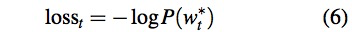
对于每⼀个time step,以输⼊序列 的 作为输⼊, 作为target,计算attention;然后⽤ Decoder得到 ,找到target对应的词在 中对应的概率 ,然后计算time step 的损失,然后加上padding mask。其中损失计算公式如下:
按如下公式计算整个序列的平均loss:
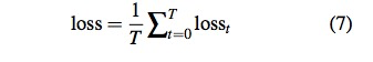
计算整个batch的平均loss并返回。
class Seq2seq(nn.Module):
    def __init__(self, v):
        super(Seq2seq, self).__init__()
        self.v = v
        self.DEVICE = config.DEVICE
        self.attention = Attention(config.hidden_size)
        self.encoder = Encoder(len(v),config.embed_size,config.hidden_size,)
        self.decoder = Decoder(len(v),config.embed_size,config.hidden_size,)
        self.reduce_state = ReduceState()


    def forward(self, x, x_len, y, len_oovs, batch, num_batches):
        """Define the forward propagation for the model.
        """
        x_copy = replace_oovs(x, self.v)
        x_padding_masks = torch.ne(x, 0).byte().float()
        encoder_output, encoder_states = self.encoder(x_copy)
        # Reduce encoder hidden states.
        decoder_states = self.reduce_state(encoder_states)
        # Calculate loss for every step.
        step_losses = []
        for t in range(y.shape[1]-1):
            # Do teacher forcing.
            x_t = y[:, t]
            x_t = replace_oovs(x_t, self.v)
            y_t = y[:, t+1]
            # Get context vector from the attention network.
            context_vector, attention_weights = self.attention(decoder_states, encoder_output, x_padding_masks, coverage_vector)
            # Get vocab distribution and hidden states from the decoder.
            p_vocab, decoder_states= self.decoder(x_t.unsqueeze(1), decoder_states, context_vector)
            # Get the probabilities predict by the model for target tokens.
            y_t = replace_oovs(y_t, self.v)
            target_probs = torch.gather(p_vocab, 1, y_t.unsqueeze(1))
            target_probs = target_probs.squeeze(1)
            # Apply a mask such that pad zeros do not affect the loss
            mask = torch.ne(y_t, 0).byte()
            # Do smoothing to prevent getting NaN loss because of log(0).
            loss = -torch.log(target_probs + config.eps)
            mask = mask.float()
            loss = loss * mask
            step_losses.append(loss)

        sample_losses = torch.sum(torch.stack(step_losses, 1), 1)
        # get the non-padded length of each sequence in the batch
        seq_len_mask = torch.ne(y, 0).byte().float()
        batch_seq_len = torch.sum(seq_len_mask, dim=1)
        # get batch loss by dividing the loss of each batch
        # by the target sequence length and mean
        batch_loss = torch.mean(sample_losses / batch_seq_len)
        return batch_loss
3. 模型优化:PGN+coverage实现
seq2seq+attention模型虽然可以自由地生成文本,但是其有很多缺点,包括但不限于:
不准确地再现事实细节
无法处理词汇表外(OOV)单词
生成重复的单词。
本节我们将对此模型做一个优化,具体而言就是实现PGN网络➕Coverage机制。
3.1 模型概览
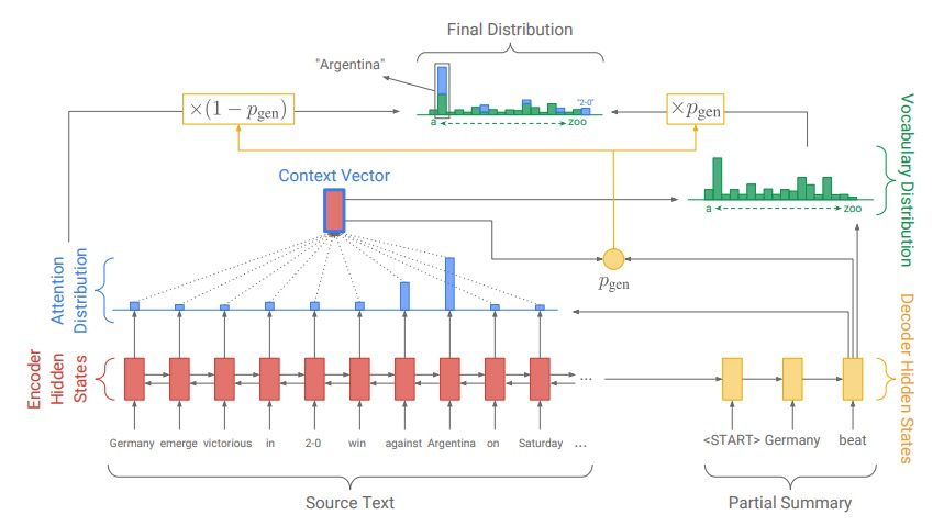
PGN +Coverage 模型框架,其优点主要有二:
PGN (指针生成器网络):一方面可以从Source文本复制token,这提高了模型对OOV单词的处理能力;另一方面也保留了生成新词的能力。所以 PGN 是一个抽取+生成的模型;
Coverage vector :对于消除重复非常有效。
模型整体框架如下图所示:
3.2 模型重点细节
前面,我们已经说过 PGN 是一个生成➕抽取的模型。更具体地,它的生成是依靠从词汇表挑选单词,它的抽取则依靠的是从Source文本复制单词。整个模型中有几个关键的细节值得我们关注:
(1)生成与抽取的把控
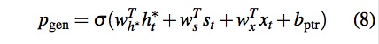
权重计算(生成概率计算):
首先,在每个解码时间步,我们会计算生成概率 ,并将这个概率用作 从词汇表挑选单词 的权重;相应地, 即为 从源文本复制单词 的权重。其中, 计算公式如下:
二者调和
然后,我们会基于生成概率对词汇分布和注意分布(注意力机制计算结果)进行加权求和,得到最终分布,并据此进行预测,公式如下:

(2)避免重复的Coverage机制
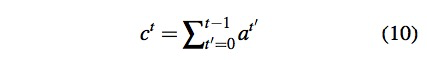
Coverage Vector:
在converage机制中,我们会更新 Coverage Vector ,它其实就是所有先前解码时间步的attention weights的总和:
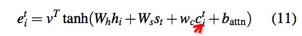
在计算Attention weight时,Converage Vector将被用作额外输入:
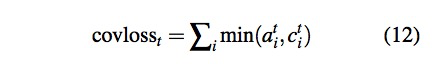
Coverage Loss
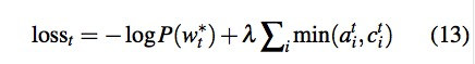
为避免同一位置被分配过多的注意力,从而减少重复,我们额外定义一个coverage loss:
3.3 模型实现细节
3.3.1 Encoder
Encoder端没有变化,这里不再赘述。
3.3.2 Decoder
多了一个实现 的计算,代码如下所示:
def forward(self, x_t, decoder_states, context_vector):
        """Define forward propagation for the decoder.
        """
        decoder_emb = self.embedding(x_t)
        decoder_output, decoder_states = self.lstm(decoder_emb, decoder_states)
        # concatenate context vector and decoder state
        decoder_output = decoder_output.view(-1, config.hidden_size)
        concat_vector = torch.cat(
            [decoder_output,
             context_vector],
            dim=-1)
        # calculate vocabulary distribution
        FF1_out = self.W1(concat_vector)
        FF2_out = self.W2(FF1_out)
        p_vocab = F.softmax(FF2_out, dim=1)
        h_dec, c_dec = decoder_states
        s_t = torch.cat([h_dec, c_dec], dim=2)
        p_gen = None
        if config.pointer:
            # Calculate p_gen.
            x_gen = torch.cat([context_vector,s_t.squeeze(0),decoder_emb.squeeze(1)], dim=-1)
            p_gen = torch.sigmoid(self.w_gen(x_gen))
        return p_vocab, decoder_states, p_gen
3.3.3 Attention
多了两部分的改进:
计算attention weights时加⼊coverage vector。
对coverage vector进⾏更新。
def forward(self, decoder_states, encoder_output, x_padding_masks, coverage_vector):
        """Define forward propagation for the attention network.
        """
        # Concatenate h and c to get s_t and expand the dim of s_t.
        h_dec, c_dec = decoder_states
        s_t = torch.cat([h_dec, c_dec], dim=2)
        s_t = s_t.transpose(0, 1)
        s_t = s_t.expand_as(encoder_output).contiguous()
        # calculate attention scores
        encoder_features = self.Wh(encoder_output.contiguous())
        decoder_features = self.Ws(s_t)
        att_inputs = encoder_features + decoder_features
        # Add coverage feature.
        if config.coverage:
            coverage_features = self.wc(coverage_vector.unsqueeze(2))  # wc c
            att_inputs = att_inputs + coverage_features
        score = self.v(torch.tanh(att_inputs))
        attention_weights = F.softmax(score, dim=1).squeeze(2)
        attention_weights = attention_weights * x_padding_masks

        # Normalize attention weights after excluding padded positions.
        normalization_factor = attention_weights.sum(1, keepdim=True)
        attention_weights = attention_weights / normalization_factor
        context_vector = torch.bmm(attention_weights.unsqueeze(1), encoder_output)
        context_vector = context_vector.squeeze(1)
        # Update coverage vector.
        if config.coverage:
            coverage_vector = coverage_vector + attention_weights
        return context_vector, attention_weights, coverage_vector
3.3.4 ReduceState
ReduceState模块也没有变化,还是用于实现数据降维。
3.3.5 get_final_distribution函数
PGN(Pointer-Generator Network) 的生成与抽取可以概括如下:
抽取(pointer):实质上就是根据 attention分布 (source 中每个 token 的概率分布\)来挑选输出的词,是从 source 中挑选最佳的 token 作为输出;
生成(generator):实质上就是依据decoder计算得到的字典概率分布 来挑选输出的词,是从字典中挑选最佳的 token 作为输出。
所以,我们可以发现 Attention 的分布和 的分布的⻓度和对应位置代表的 token 是不⼀样的。那么,在计算 final distribution 的时候为了将两个分布对应上,需要做如下处理:
先对 进⾏扩展,将 source 中的 oov 添 加到 的尾部,得到 ;这样 attention weights 中的每⼀个 token 都能在 中找到对应的位置;
然后将对应的 attention weights 叠加到扩展后的 中的对应位置,得到 final distribution。
def get_final_distribution(self, x, p_gen, p_vocab, attention_weights, max_oov):
        """Calculate the final distribution for the model.
        """
        batch_size = x.size()[0]
        # Clip the probabilities.
        p_gen = torch.clamp(p_gen, 0.001, 0.999)
        # Get the weighted probabilities.
        p_vocab_weighted = p_gen * p_vocab
        attention_weighted = (1 - p_gen) * attention_weights

        # Get the extended-vocab probability distribution
        extension = torch.zeros((batch_size, max_oov)).float().to(self.DEVICE)
        p_vocab_extended = torch.cat([p_vocab_weighted, extension], dim=1)
        # Add the attention weights to the corresponding vocab positions.
        final_distribution =  p_vocab_extended.scatter_add_(dim=1, index=x, src=attention_weighted)
        return final_distribution
3.3.6 PGN的整体前向传导
与Seq2seq+attention相比,PGN的整体前向传导只是多了一个计算Converage Loss 的过程。
def forward(self, x, x_len, y, len_oovs, batch, num_batches):
        """Define the forward propagation for the model.
        """
        x_copy = replace_oovs(x, self.v)
        x_padding_masks = torch.ne(x, 0).byte().float()
        encoder_output, encoder_states = self.encoder(x_copy)
        # Reduce encoder hidden states.
        decoder_states = self.reduce_state(encoder_states)
        # Initialize coverage vector.
        coverage_vector = torch.zeros(x.size()).to(self.DEVICE)
        # Calculate loss for every step.
        step_losses = []
        for t in range(y.shape[1]-1):
            # Do teacher forcing.
            x_t = y[:, t]
            x_t = replace_oovs(x_t, self.v)

            y_t = y[:, t+1]
            # Get context vector from the attention network.
            context_vector, attention_weights, next_coverage_vector = \
                self.attention(decoder_states,
                               encoder_output,
                               x_padding_masks,
                               coverage_vector)
            # Get vocab distribution and hidden states from the decoder.
            p_vocab, decoder_states, p_gen = self.decoder(x_t.unsqueeze(1),
                                                          decoder_states,
                                                          context_vector)

            final_dist = self.get_final_distribution(x,
                                                     p_gen,
                                                     p_vocab,
                                                     attention_weights,
                                                     torch.max(len_oovs))

            # Get the probabilities predict by the model for target tokens.
            target_probs = torch.gather(final_dist, 1, y_t.unsqueeze(1))
            target_probs = target_probs.squeeze(1)

            # Apply a mask such that pad zeros do not affect the loss
            mask = torch.ne(y_t, 0).byte()
            # Do smoothing to prevent getting NaN loss because of log(0).
            loss = -torch.log(target_probs + config.eps)

            # Add coverage loss.
            ct_min = torch.min(attention_weights, coverage_vector)
            cov_loss = torch.sum(ct_min, dim=1)
            loss = loss + config.LAMBDA * cov_loss
            coverage_vector = next_coverage_vector

            mask = mask.float()
            loss = loss * mask
            step_losses.append(loss)

        sample_losses = torch.sum(torch.stack(step_losses, 1), 1)
        # get the non-padded length of each sequence in the batch
        seq_len_mask = torch.ne(y, 0).byte().float()
        batch_seq_len = torch.sum(seq_len_mask, dim=1)

        # get batch loss by dividing the target sequence length and mean
        batch_loss = torch.mean(sample_losses / batch_seq_len)
        return batch_loss

在这里插入代码片
4. 模型训练+可视化
4.1 pytorch训练模板
optimizer = None # Choose an optimizer from torch.optim
batch_losses = []
for batch in batches:
    model.train() # Sets the module in training mode.
    optimizer.zero_grad() # Clear gradients.
    batch_loss = model(**params)# Calculate loss for a batch.
    batch_losses.append(loss.item())
    batch_loss.backward() # Backpropagation.
    optimizer.step() # Update weights.
epoch_loss = torch.mean(batch_losses)
4.2 TensorBoard可视化
创建⼀个SummaryWriter对象,调⽤
add_scalar函数来记录损失,记得写完要调⽤close函数。并且在适当的位置实现梯度剪裁(
clip_grad_norm_函数)。
整体的代码如下:
optimizer = optim.Adam(model.parameters(), lr=config.learning_rate)
    writer = SummaryWriter(config.log_path)
    # tqdm: A tool for drawing progress bars during training.
    with tqdm(total=config.epochs) as epoch_progress:
        for epoch in range(start_epoch, config.epochs):
            batch_losses = []  # Get loss of each batch.
            num_batches = len(train_dataloader)
            with tqdm(total=num_batches//100) as batch_progress:
                for batch, data in enumerate(tqdm(train_dataloader)):
                    x, y, x_len, y_len, oov, len_oovs = data
                    model.train()  # Sets the module in training mode.
                    optimizer.zero_grad()  # Clear gradients.
                    # Calculate loss.
                    loss = model(x, x_len, y, len_oovs, batch=batch, num_batches=num_batches)
                    batch_losses.append(loss.item())
                    loss.backward()  # Backpropagation.
                    # Do gradient clipping to prevent gradient explosion.
                    clip_grad_norm_(model.encoder.parameters(),
                                    config.max_grad_norm)
                    clip_grad_norm_(model.decoder.parameters(),
                                    config.max_grad_norm)
                    clip_grad_norm_(model.attention.parameters(),
                                    config.max_grad_norm)
                    optimizer.step()  # Update weights.
                    # Output and record epoch loss every 100 batches.
                    if (batch % 100) == 0:
                        batch_progress.set_description(f'Epoch {epoch}')
                        batch_progress.set_postfix(Batch=batch,
                                                   Loss=loss.item())
                        batch_progress.update()
                        # Write loss for tensorboard.
                        writer.add_scalar(f'Average loss for epoch {epoch}',
                                          np.mean(batch_losses),
                                          global_step=batch)
            # Calculate average loss over all batches in an epoch.
            epoch_loss = np.mean(batch_losses)
            epoch_progress.set_description(f'Epoch {epoch}')
            epoch_progress.set_postfix(Loss=epoch_loss)
            epoch_progress.update()
            avg_val_loss = evaluate(model, val_data, epoch)
            print('training loss:{}'.format(epoch_loss), 'validation loss:{}'.format(avg_val_loss))

    writer.close()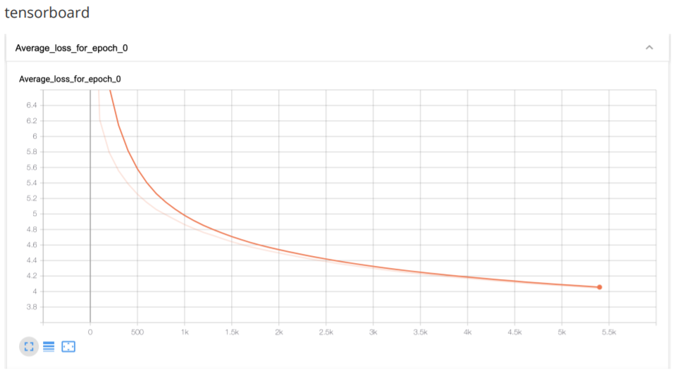
5. 模型解码
5.1 Greedy search实现
基于贪心思想的 Greedy Search 实现整体上⽐较简单,⽤ Encoder 编码输⼊,然后将每⼀个 time step 的信息传递给 Decoder,计算attention,得到 Decoder 的 ,根据 选出概率最⼤的词作为下⼀个token。
代码如下:
def greedy_search(self,
                      x,
                      max_sum_len,
                      len_oovs,
                      x_padding_masks):
        """Function which returns a summary by always picking
        """

        # Get encoder output and states.
        encoder_output, encoder_states = self.model.encoder(
            replace_oovs(x, self.vocab))

        # Initialize decoder's hidden states with encoder's hidden states.
        decoder_states = self.model.reduce_state(encoder_states)

        # Initialize decoder's input at time step 0 with the SOS token.
        x_t = torch.ones(1) * self.vocab.SOS
        x_t = x_t.to(self.DEVICE, dtype=torch.int64)
        summary = [self.vocab.SOS]
        coverage_vector = torch.zeros((1, x.shape[1])).to(self.DEVICE)
        # Generate hypothesis with maximum decode step.
        while int(x_t.item()) != (self.vocab.EOS) \
                and len(summary) < max_sum_len:
            context_vector, attention_weights, coverage_vector = \
                self.model.attention(decoder_states,
                                     encoder_output,
                                     x_padding_masks,
                                     coverage_vector)
            p_vocab, decoder_states, p_gen = \
                self.model.decoder(x_t.unsqueeze(1),
                                   decoder_states,
                                   context_vector)
            final_dist = self.model.get_final_distribution(x,
                                                           p_gen,
                                                           p_vocab,
                                                           attention_weights,
                                                           torch.max(len_oovs))
            # Get next token with maximum probability.
            x_t = torch.argmax(final_dist, dim=1).to(self.DEVICE)
            decoder_word_idx = x_t.item()
            summary.append(decoder_word_idx)
            x_t = replace_oovs(x_t, self.vocab)
        return summary
5.2 Beam search实现与优化
我们对 Beam search 进行了优化,主要是加入了 Length normalization, Coverage normalization以及End of sentence normalization。
Beam search 的实现大体可以分为三步:
首先,首先定义一个
Beam类,作为一个存放候选序列的容器,属性需维护当前序列中的 token 以及对应的对数概率,同时还需维护跟当前 timestep 的 Decoder 相关的一些变量。此外,还需要给 Beam 类实现两个函数:
一个
extend函数用以扩展当前的序列(即添加新的 time step的 token 及相关变量);一个
score函数用来计算当前序列的分数(在Beam类下的seq_score函数中有Length normalization以及Coverage normalization)。
class Beam(object):
    def __init__(self,
                 tokens,
                 log_probs,
                 decoder_states,
                 coverage_vector):
        self.tokens = tokens
        self.log_probs = log_probs
        self.decoder_states = decoder_states
        self.coverage_vector = coverage_vector

    def extend(self,
               token,
               log_prob,
               decoder_states,
               coverage_vector):
        return Beam(tokens=self.tokens + [token],
                    log_probs=self.log_probs + [log_prob],
                    decoder_states=decoder_states,
                    coverage_vector=coverage_vector)
    def seq_score(self):
        """
        This function calculate the score of the current sequence.
        """
        len_Y = len(self.tokens)
        # Lenth normalization
        ln = (5+len_Y)**config.alpha / (5+1)**config.alpha
        cn = config.beta * torch.sum(  # Coverage normalization
            torch.log(
                config.eps +
                torch.where(
                    self.coverage_vector < 1.0,
                    self.coverage_vector,
                    torch.ones((1, self.coverage_vector.shape[1])).to(torch.device(config.DEVICE))
                )
            )
        )
        score = sum(self.log_probs) / ln + cn
        return score
接着,实现一个
best_k函数,作用是将一个 Beam 容器中当前 time step 的变量传入 Decoder 中,计算出新一轮的词表概率分布,并从中选出概率最大的 k 个 token 来扩展当前序列(其中加入了End of sentence normalization),得到 k 个新的候选序列。
def best_k(self, beam, k, encoder_output, x_padding_masks, x, len_oovs):
        """Get best k tokens to extend the current sequence at the current time step.
        """
        # use decoder to generate vocab distribution for the next token
        x_t = torch.tensor(beam.tokens[-1]).reshape(1, 1)
        x_t = x_t.to(self.DEVICE)

        # Get context vector from attention network.
        context_vector, attention_weights, coverage_vector = \
            self.model.attention(beam.decoder_states,
                                 encoder_output,
                                 x_padding_masks,
                                 beam.coverage_vector)
、
        p_vocab, decoder_states, p_gen = \
            self.model.decoder(replace_oovs(x_t, self.vocab),
                               beam.decoder_states,
                               context_vector)

        final_dist = self.model.get_final_distribution(x,
                                                       p_gen,
                                                       p_vocab,
                                                       attention_weights,
                                                       torch.max(len_oovs))
        # Calculate log probabilities.
        log_probs = torch.log(final_dist.squeeze())
        # EOS token penalty. Follow the definition in
        log_probs[self.vocab.EOS] *= \
            config.gamma * x.size()[1] / len(beam.tokens)
        log_probs[self.vocab.UNK] = -float('inf')
        # Get top k tokens and the corresponding logprob.
        topk_probs, topk_idx = torch.topk(log_probs, k)
        best_k = [beam.extend(x,
                  log_probs[x],
                  decoder_states,
                  coverage_vector) for x in topk_idx.tolist()]
        return best_k
最后我们实现主函数
beam_search。初始化encoder、attention和decoder的输⼊。然后,对于每⼀个解码步,对现有的 个beam,我们分别利⽤best_k函数来得到各⾃最佳的 个extended beam,也就是每个解码步我们会得到 个新的beam,然后只保留分数最⾼的 个,作为下⼀轮需要扩展的 个beam。为了只保留分数最⾼的 个beam,我们可以⽤⼀个堆(heap)来实现,堆的中只保存 个节点,根结点保存分数最低的beam。
def beam_search(self,
                    x,
                    max_sum_len,
                    beam_width,
                    len_oovs,
                    x_padding_masks):
        """Using beam search to generate summary.
        """
        # run body_sequence input through encoder
        encoder_output, encoder_states = self.model.encoder(
            replace_oovs(x, self.vocab))
        coverage_vector = torch.zeros((1, x.shape[1])).to(self.DEVICE)
        # initialize decoder states with encoder forward states
        decoder_states = self.model.reduce_state(encoder_states)
        # initialize the hypothesis with a class Beam instance.
        init_beam = Beam([self.vocab.SOS],
                         [0],
                         decoder_states,
                         coverage_vector)
        k = beam_width
        curr, completed = [init_beam], []
        # use beam search for max_sum_len (maximum length) steps
        for _ in range(max_sum_len):
            # get k best hypothesis when adding a new token
            topk = []
            for beam in curr:
                # When an EOS token is generated, add the hypo to the completed
                if beam.tokens[-1] == self.vocab.EOS:
                    completed.append(beam)
                    k -= 1
                    continue
                for can in self.best_k(beam,
                                       k,
                                       encoder_output,
                                       x_padding_masks,
                                       x,
                                       torch.max(len_oovs)
                                       ):
                    # Using topk as a heap to keep track of top k candidates.
                    add2heap(topk, (can.seq_score(), id(can), can), k)

            curr = [items[2] for items in topk]
            # stop when there are enough completed hypothesis
            if len(completed) == beam_width:
                break
        completed += curr
        # sort the hypothesis by normalized probability and choose the best one
        result = sorted(completed,
                        key=lambda x: x.seq_score(),
                        reverse=True)[0].tokens
        return result
6. Rouge评估
在本次项目中使用ROUGE-1、ROUGE-2以及ROUGE-L评估。
rouge直接调用了库函数。整体评估流程如下:首先建立自带的ROUGE容器初始化;然后预测函数得到我们的生成文本,将他们Build hypotheses;最后比较答案得到分数。
class RougeEval():
    def __init__(self, path):
        self.path = path
        self.scores = None
        self.rouge = Rouge()
        self.sources = []
        self.hypos = []
        self.refs = []
        self.process()
    def process(self):
        print('Reading from ', self.path)
        with open(self.path, 'r') as test:
            for line in test:
                source, ref = line.strip().split('<sep>')
                ref = ''.join(list(jieba.cut(ref))).replace('。', '.')
                self.sources.append(source)
                self.refs.append(ref)
        print(f'Test set contains {len(self.sources)} samples.')


    def build_hypos(self, predict):
        print('Building hypotheses.')
        count = 0
        for source in self.sources:
            count += 1
            if count % 100 == 0:
                print(count)
            self.hypos.append(predict.predict(source.split()))

    def get_average(self):
        assert len(self.hypos) > 0, 'Build hypotheses first!'
        print('Calculating average rouge scores.')
        return self.rouge.get_scores(self.hypos, self.refs, avg=True)

    def one_sample(self, hypo, ref):
        return self.rouge.get_scores(hypo, ref)[0]
rouge_eval = RougeEval(config.test_data_path)
predict = Predict()
rouge_eval.build_hypos(predict)
result = rouge_eval.get_average()
print('rouge1: ', result['rouge-1'])
print('rouge2: ', result['rouge-2'])
print('rougeL: ', result['rouge-l'])
7. 数据增强
NLP领域经常面临少样本问题,尤其是在金融或者医疗等垂直领域,更是缺乏高质量的标注语料。
在少样本场景下,我们常常会用到数据增强。本节将实现以下几种数据增强的技术:单词替换,回译,半监督学习。
7.1 单词替换
中文不像英文中有 WordNet 这种成熟的近义词词典可以使用,所以我们选择在 embedding 的词向量空间中寻找语义最接近的词。
通过使用在大量数据上预训练好的中文词向量,我们可以到每个词在该词向量空间中语义最接近的词,然后替换原始样本中的词,得到新的样本。但是有一个问题是,如果我们替换了样本中的核心词汇,比如将文案中的体现关键卖点的词给替换掉了,可能会导致核心语义的丢失。
对此,我们有两种解决办法:
通过 tfidf 权重对词表里的词进行排序,然后替换排序靠后的词;
先通过无监督的方式挖掘样本中的主题词,然后只替换不属于主题词的词汇。
任务1,extract_keywords函数。
根据TFIDF确认需要排除的核⼼词汇。
def extract_keywords(self, dct, tfidf, threshold=0.2, topk=5):
        """find high TFIDF socore keywords
        """
        tfidf = sorted(tfidf, key=lambda x: x[1], reverse=True)
        return list(islice(
            [dct[w] for w, score in tfidf if score > threshold], topk
))任务2,replace函数。
embedding 的词向量空间中寻找语义最接近的词进⾏替换。
def replace(self, token_list, doc):
        """replace token by another token which is similar in wordvector
        """
        keywords = self.extract_keywords(self.dct, self.tfidf_model[doc])
        num = int(len(token_list) * 0.3)
        new_tokens = token_list.copy()
        while num == int(len(token_list) * 0.3):
            indexes = np.random.choice(len(token_list), num)
            for index in indexes:
                token = token_list[index]
                if isChinese(token) and token not in keywords and token in self.wv:
                    new_tokens[index] = self.wv.most_similar(
                        positive=token, negative=None, topn=1
                        )[0][0]
            num -= 1
return ' '.join(new_tokens)任务3,generate_samples函数。
def generate_samples(self, write_path):
        """generate new samples file
        """
        replaced = []
        count = 0
        for sample, token_list, doc in zip(self.samples, self.refs, self.corpus):
            count += 1
            if count % 100 == 0:
                print(count)
                write_samples(replaced, write_path, 'a')
                replaced = []
            replaced.append(
                sample.split('<sep>')[0] + ' <sep> ' + self.replace(token_list, doc)
                )
替换全部的reference,和对应的source形成新样本
7.2 回译
我们可以使用成熟的机器翻译模型,将中文文本翻译成一种外文,然后再翻译回中文,由此可以得到语义近似的新样本。
比如,利⽤百度 translate API 接⼝将 source 、reference 翻译成英语,再由英语翻译成汉语,形成新样本。具体请参看百度翻译官网[1]。另外不同的语⾔样本的训练效果会有所不同,建议多尝试⼏种中间语⾔,⽐如⽇语等。
任务1:translate函数
建⽴http连接,发送翻译请求,以及接收翻译结果。关于这⼀部分可以参考百度接⼝ translate API 的demo。
def translate(q, source, target):
    """translate q from source language to target language
    """
    #  refer to the official documentation   https://api.fanyi.baidu.com/
    # There are demo on the website ,  register on the web site ,and get AppID, key, python3 demo.
    appid = ''  # Fill in your AppID
    secretKey = ''  # Fill in your key
    httpClient = None
    myurl = '/api/trans/vip/translate'
    fromLang = source  # The original language
    toLang = target  # The target language
    salt = random.randint(32768, 65536)
    sign = appid + q + str(salt) + secretKey
    sign = hashlib.md5(sign.encode()).hexdigest()
    myurl = '/api/trans/vip/translate' + '?appid=' + appid + '&q=' + urllib.parse.quote(
        q) + '&from=' + fromLang + '&to=' + toLang + '&salt=' + str(
        salt) + '&sign=' + sign
    try:
        httpClient = http.client.HTTPConnection('api.fanyi.baidu.com')
        httpClient.request('GET', myurl)
        # response is HTTPResponse object
        response = httpClient.getresponse()
        result_all = response.read().decode("utf-8")
        result = json.loads(result_all)
        return result
    except Exception as e:
        print(e)
    finally:
        if httpClient:
httpClient.close()任务2:back_translate函数
对数据进⾏回译。
def back_translate(q):
    """back_translate
    """
    en = translate(q, "zh", 'en')['trans_result'][0]['dst']
    time.sleep(1.5)
    target = translate(en, "en", 'zh')['trans_result'][0]['dst']
    time.sleep(1.5)
    return target
7.3 自助式样本生成
当训练出一个文本生成模型后,我们可以利用训练好的模型为我们原始样本中的 reference 生成新的 source,并作为新的样本继续训练我们的模型。
semi_supervised 函数
我们可以使⽤训练好的 PGN 模型将reference送⼊模型,⽣成新的source:
def semi_supervised(samples_path, write_path, beam_search):
    """use reference to predict source
    """
    pred = Predict()
    print('vocab_size: ', len(pred.vocab))
    # Randomly pick a sample in test set to predict.
    count = 0
    semi = []
    with open(samples_path, 'r') as f:
        for picked in f:
            count += 1
            source, ref = picked.strip().split('<sep>')
            prediction = pred.predict(ref.split(), beam_search=beam_search)
            semi.append(prediction + ' <sep> ' + ref)
            if count % 100 == 0:
                write_samples(semi, write_path, 'a')
                semi = []
下面是一个样例:
# source 文本
帕莎 太阳镜 男⼠ 太阳镜 偏光 太阳眼镜 墨镜 潮 典雅 灰 颜⾊ 选择 , 细节 特⾊ 展示 , ⻆度 展示 , ⻛ 尚 演 , ⾦属, 透光 量 , 不易 变形 , 坚固耐⽤ , 清晰 柔和 , 镜⽚ 材质 , 尼⻰ ⾼ , 型号 , 镜架 材质 , ⾦属 镜腿 , 镜布 镜盒 , ⿐ 间距 , 轻盈 ⿐托 , 品牌 刻印 , ⽆缝 拼接 眼镜 配件类型 镜盒 功 能 偏光 类型 偏光太阳镜 镜⽚材质 树脂 ⻛格 休闲⻛ 上市时间 2016年夏季 镜框形状 ⽅形 适⽤性别 男 镜架材质 合⾦

# reference文本
夏天 到 了 , 在 刺眼 的 阳光 下 少不了 这 款 时尚 的 男⼠ 太阳镜 ! 时尚 的 版型 , 适⽤ 各种 脸型 , 突出 您 的 型 男 ⻛范 。 其⾼ 镍 ⾦属 材质 的 镜架 , ⼗分 的 轻盈 , 带给 您 舒适 的 佩戴 体验 。

# 将reference送⼊模型后⽣成的数据new source:

版型 设计 , 时尚 百搭 , 适合 多种 场合 佩戴 。 时尚 ⾦属 拉链 , 经久耐⽤ 。 带给 你 舒适 的 佩戴 体验 。 ⻛范 与 铰链 的 镜架 , 舒适 耐磨 , 不易 变形 。 带给 你 意想不到 的 修身 效果 , 让 你 的 夏 季 充满 着 不 ⼀样 的 魅⼒ , 让 这个 夏天 格外 绚烂 , 让 这个 夏天 格外 绚烂 。 时尚 的 版型 , 让 你 穿 起来 更 有 男⼈味 , 让 这个 夏天格外 绚烂 绚烂 , 让 这个 夏天 格外 绚烂 。 时尚 的 版型 , 让 你 穿 起来 更 有 男⼈味 , 让 这个 夏天 格外 绚烂 绚烂 , 是 秋装 上 上 之选 。
8. 优化技巧
在 Seq2seq 模型中,由于 Decoder 在预测阶段需要根据上一步的输出来生成当前步输出,所以会面临Exposure bias的问题。
所谓 Exposure bias(暴露偏差) 简单地理解就是:在训练阶段我们使用 ground truth 作为 Decoder 的输入(称之为 Teacher forcing), 但预测阶段却只能使用 Decoder 上一步的输出,导致输入样本分布不一样,而影响 Decoder 的表现。
对此,我们有两种技巧进行优化:
Weight Tying
Scheduled Sampling
8.1 Weight tying
Weight tying 即共享 Encoder 和 Decoder 的 embedding 权重矩阵,使得其输入的词向量表达具有一致性。
这里我们使⽤的是three-way tying,即Encoder的input embedding、Decoder的input emdedding和Decoder的output embedding之间的权重共享。
Encoder端需要加入如下代码:
if config.weight_tying:
            embedded = decoder_embedding(x)
        else:
            embedded = self.embedding(x)
Decoder端在output中加入如下代码:
if config.weight_tying:
            FF2_out = torch.mm(FF1_out, torch.t(self.embedding.weight))
        else:
            FF2_out = self.W2(FF1_out)
8.2 Scheduled Sampling
Scheduled Sampling 即在训练阶段,将 ground truth 和 Decoder 的输出混合起来用作下一个 time step 的 Decoder 的输入。
具体的做法是每个 time step 以一个 的概率进行 Teacher forcing,以 的概率不进行 Teacher forcing。 的大小可以随着 batch 或者 epoch 衰减,比如开始训练的阶段完全使用 groud truth 以加快模型收敛,到后面逐渐将 ground truth 替换成模型自己的输出,到训练后期就与预测阶段的输出一致了。
代码很简单,如下所示:进入每个epoch都要去确定是否要进行teacher_forcing。可以通过epoch或者batch数控制按照⼀定的概率给出是否需要进⾏teacher forcing的指示。
class ScheduledSampler():
    def __init__(self, phases):
        self.phases = phases
        self.scheduled_probs = [i / (self.phases - 1) for i in range(self.phases)]

    def teacher_forcing(self, phase):
        """According to a certain probability to choose whether to execute teacher_forcing
        """
        sampling_prob = random.random()
        if sampling_prob >= self.scheduled_probs[phase]:
            return True
        else:
            return False
如果epoch=0,那么百分之百进行Teacher forcing,如果epoch=num_eopch-1,那么百分之零进行Teacher forcing。
9. 实验结果
下面实验结果大家可以作为一个参考:
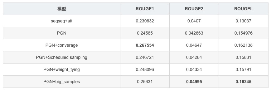
对于不同数据不同任务不同超参数可能会有差异,不过也大致反映了一些规律。通过实验比对,个人感觉优化效果最好的是Converage和数据增广。
参考资料
[1]
百度翻译官网: https://api.fanyi.baidu.com/
文章来源:https://blog.csdn.net/qq_38556984/article/details/108294319
作者:fond_dependent
编辑:@公众号:AI算法小喵
📝论文解读投稿,让你的文章被更多不同背景、不同方向的人看到,不被石沉大海,或许还能增加不少引用的呦~ 投稿加下面微信备注“投稿”即可。
最近文章
苏州大学NLP团队文本生成&预训练方向招收研究生/博士生(含直博生)
投稿或交流学习,备注:昵称-学校(公司)-方向,进入DL&NLP交流群。
方向有很多:机器学习、深度学习,python,情感分析、意见挖掘、句法分析、机器翻译、人机对话、知识图谱、语音识别等。

记得备注~


 653
653


 被折叠的 条评论
为什么被折叠?
被折叠的 条评论
为什么被折叠?
 到【灌水乐园】发言


