实现累加求和_Seq2Seq+PGN实现文本摘要生成自整理

Pre：

例行吐槽知乎上传doc的格式错乱。。。

一、概述

1、概述

Topic：文本摘要

Baseline：Seq2Seq+Attention的文本生成模型

模型优化：抽取式+生成式 PGN网络及Coverage机制优化

数据源：电商平台上的营销文本，文本分为三部分

• 商品标题
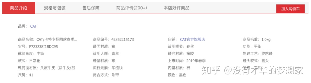
• 商品参数
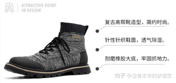
• 商品宣传图片中的宣传文案
• 选用回译、替换等方法进行小规模的数据增强

训练优化：Scheduled Sampling、Weight Tying

数据生成方式：Beam-Search及优化

数据输出：一段营销文案句子

模型评估：Rouge-1、Rouge-2、Rouge-L

参考论文：第一篇是最主要的，基本是复现

（1）ACL2017：《Get To The Point: Summarization with Pointer-Generator Networks》

（2）CiKM2018：《Multi-Source Pointer Network for Product Title Summarization》

（3）ACL2016：《Incorporating Copying Mechanism in Sequence-to-Sequence Learning》

2、原始数据展示：

1、商品标题

2、商品部分参数

3、营销图片中的文案（人为撰写的作为reference）

二、理论部分

这部分对概述中提到的所有相关知识做一个整理

1、Seq2Seq+Attention模型

Seq2Seq模型简单概括就是拼接两个RNN系的模型，分别称为模型的Encoder部分和Decoder部分

Encoder部分负责输入文本语义的编码，生成一个“浓缩输入语义”的语义空间meaning space

Decoder部分负责根据这个语义空间及每个time-step的Decoder输出，进行Attention机制并生成句子

从而实现在语义背景下从句子到句子的直接转换（Sequence to Sequence），而区别于以往单个单词单个单词的对照输出

模型架构如图所示：

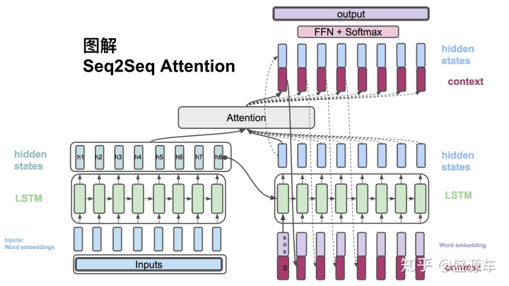
Encoder和Decoder都由RNN系的模型拼接而成，因此能够进行序列化的编码和输出，通常使用LSTM或Bi-LSTM来尽量减少梯度消失和梯度爆炸的问题，保证生成的效果更加的理想

Attention机制是Seq2Seq的核心，思路是根据Encoder的每个hidden state生成一个权重，之后经过归一化，得到一个新的权重，从而根据这个权重更新Meaning-Space的向量，之后与Decoder进行运算，输出结果

具体说来，每一部分的计算过程可以概述如下：

Encoder：接受的是每一个单词的embedding，和上一个时间点的hidden state。输出的是这个时间点的hidden state。

Attention：对Encoder的hidden state进行运算，得到中间的Attention层并以此形成Meaning Space

Decoder：

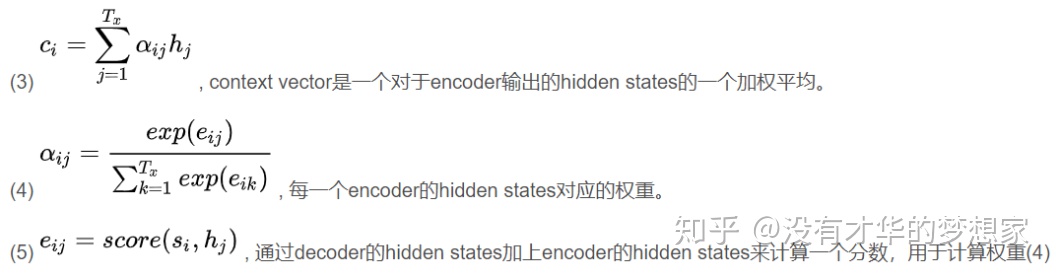
• 通过Decoder每一个time step 的hidden state与Encoder的hidden state计算一个权重，做归一化处理得到与每一个Encoder的hidden state的权重/得分，根据这个对应权重与hidden state拼接、加权平均得到Context Vector。
• 之后这个Context Vector与Decoder部分的前一个time step的hidden state拼接起来，计算得到当前步Decoder的输出，并作为下一个time step的输入，如此循环往复，直到输出最终结果。
• 需要注意的是，训练阶段Decoder部分每一步的输入用的是Reference文本，也即其实是一个“已知答案的假预测”，为的是使模型能够更快的拟合当前的训练样本，但在后期也应该使用真实的输出作为下一步的输入，这个地方在后续训练的优化部分会讲到

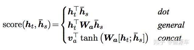
最后，阐述一下Attention的计算方式，也即Decoder中Context vector的计算方式，论文中给出的三种计算方式分别为：

（1）点乘（dot）

输入是：

• Encoder的所有hidden state（H），大小为(hidden dim, sequence length)
• Decoder在前一步的hidden state（S），大小为（hidden dim, 1）

计算：旋转H与S做点乘得到一个大小为(sequence length, 1)的分数score，做归一化得到权重α

输出：将H与α做点乘，也即加权平均得到context vector输出

（2）general方式

输入是：

• Encoder的所有hidden state（H），大小为(hidden dim1, sequence length)
• Decoder在前一步的hidden state（S），大小为（hidden dim2, 1）
• 这里的hidden dim1与hidden dim2并不一样

计算：旋转H(sequence length,hidden dim1)与Wa(hidden dim1,hidden dim2)做点乘，再和S做点乘，得到一个大小为(sequence length, 1)的分数score，做归一化得到权重α

输出：将H与α做点乘，也即加权平均得到context vector输出

（3）Concat方式

为了简便，这里直接贴三种方式的score计算公式，其余部分都一样：

模型的优缺点：

想明白了模型的优缺点，才知道我们需要在这个baseline上如何做改动

最大的好处是部分解决了梯度的问题，传统RNN的信息包含在最后一个信息元中，而随着梯度消失、序列长度增加，很有可能最后一个信息元考虑不到序列前面的信息，而加了attention之后所有的信息都有可能被考虑到，因此更好

还有一个好处是增强了模型的可解释性，以往的RNN计算不太能够知道“错在哪里”，但由于加了attention，可以知道当前哪个权值是最大的，从而分析错误可能由他引起，或者能够发现当前attention权重最大的点不应该在当前的单词，也就能找到错误的根源

而模型的缺点则是在Attention里求score的方法，不难想到这种机制的前提假设最好要求Encoder中的不同的hidden state要相对独立（能够表示不同的信息是最好的），但由LSTM的性质又知道，hidden state是一定不是独立的，且一定考虑到了之前的hidden state，这由我们的实际经验也可以分析出来，因此这也带来了较大的冗余度

2、PGN网络及其要解决的问题

回顾Seq2Seq网络我们可以发现，不管是哪种Attention计算方式，最终的目的都是得到一个概率，选择概率最大的wordid，然后去词表中找单词，实现index2word，最终输出单词

但是这种方式在实际使用的过程中存在着三个缺点：

• 无法生成OOV单词，只能生成词汇表中的词
• 会产生错误的事实，比如姓名之间错误
• 自我重复，即聚焦于某些公共Attention很大的单词，从而重复输出

PGN网络主要解决的是第一个问题，也即使用一种混合的指针生成网络，他能够从源端复制单词，也能够从词表当中去生成词语。前者称为抽取式，后者称为生成式。

这里重点讲这种抽取式网络，其实就是在做attention时，分别对每一个Encoder的hidden_state做attention（这里的计算不变，区别在于对单点计算，不累加），之后选取attention_weight值最大的那个作为当前Decoder节点的输出，从而使得输出集合是输入集合的子集

主要与生成式网络的区别在于：

• Decoder的输出不再是遍历词表
• 用attention_weight作为评判标准
• 输出一定是输入的子集，即这种方式下输出词汇一定在输入序列的集合中，在一定程度上避免了OOV的问题
• 以往的生成式模型：自由、灵活但不是很可控
• 抽取式网络相对可控，确切的说是将信息来源限制在输入的信息范围中

接下来我们结合PGN的几篇论文具体的阐述他的实现机制

1、ACL2017：《Get To The Point: Summarization with Pointer-Generator Networks》

这篇也是本文最主要参考并做了复现的论文

论文使用的是两个模型叠加起来的PGN：

• 第一个还是传统的Seq2Seq模型，基于的是全局的词表
• 第二个是Pointer-Network，基于的是source-word这个小表

令最终的输出概率为二者概率的加权平均，并能够做动态调整，公式如下：

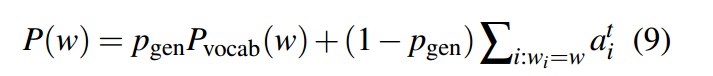
Attention_weight求和表示的是对一个句子中相同单词的attention进行累加

具体这个P_gen的计算公式是：

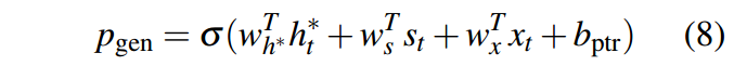
其中的四个变量分别是：h_t：context vector、s_t：decoder的hidden state、x_t：上一步的输出，b：偏置

因此，模型的整体架构为：

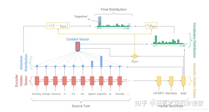
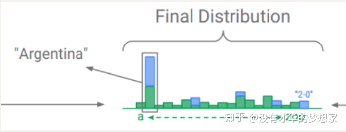
这里还可以看到final distribution中部分点是没有蓝色的，这是因为本来source_text就是整个词表的子集罢了，当然只有部分是有概率的，只需要将有的相加就可以了

对于OOV的问题，就像Souce-Text中的2：0，这个最后就只有来自于Pointer-Network的概率，没有来自于传统Seq2Seq的

这里也允许有多个UNK，因为我们在Pointer-Network中肯定是知道的，在预处理时单独把它记录出来即可

2、CiKM2018：《Multi-Source Pointer Network for Product Title Summarization》

这是一篇阿里的团队写的文本摘要任务的文章，具体场景是生成商品的标题摘要信息

这篇文章的PGN是将两个抽取式网络拼接起来，从而生成摘要，从输出是输入的子集这一性质我们也很容易想到这个应用

网络的结构：

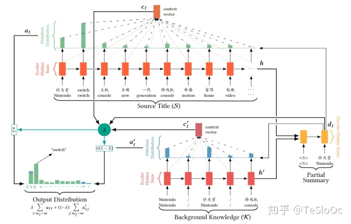
可以看到分别对两个LSTM网络进行抽取，一个的信息S是商品的标题，另一个K是商品的背景信息、

3、ACL2016：《Incorporating Copying Mechanism in Sequence-to-Sequence Learning》

这是一篇港大和华为诺亚方舟实验室生产的论文

本文的模型通过借鉴人类在处理难理解的文字时采用的死记硬背的方法，提出了COPYNET。将拷贝模式融入到了Seq2Seq模型中，将传统的生成模式和拷贝模式混合起来构建了新的模型，非常好地解决了OOV问题。

Decoder部分越来越复杂，从而取得一个比较好的效果

关于这篇文章的一个容易想到的场景是在类似于对话机器人的场景中，直接复制重要信息，如：

---“hello，我是xxx”

---“xxx你好，我是Siri”（这里的xxx就是可以直接复制粘贴的对象）

模型CopyNet的架构如下：

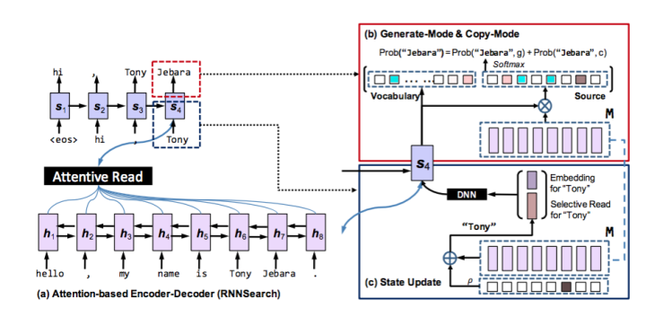
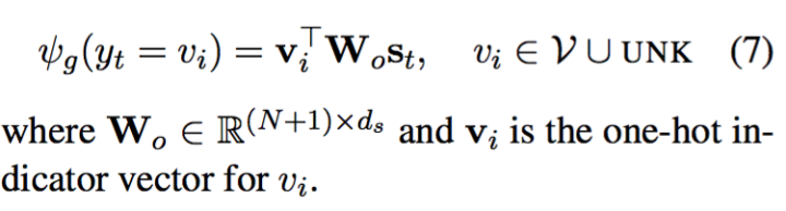
文章中将所有的单词分为以下四种分类：

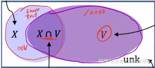
并根据这四种情况来判定最终生成单词的概率，具体的公式如下：

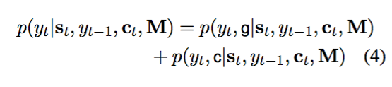
g是generate生成模式，c是copy拷贝模式，两种模式的概率计算公式由单词分布在四种情况之下哪一种不同

将上图的公式放到第一张图里可能会更加直观：

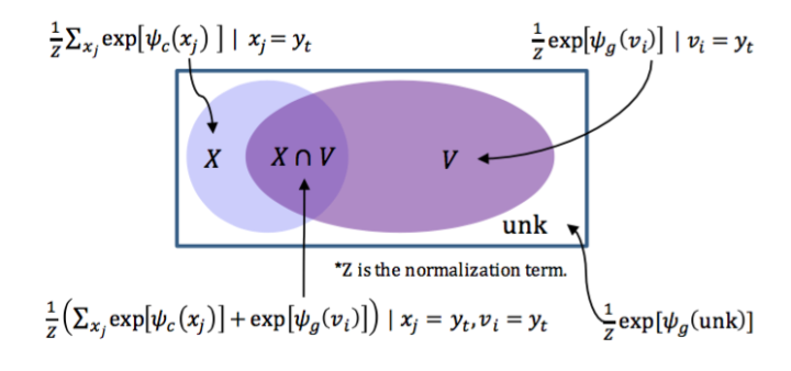
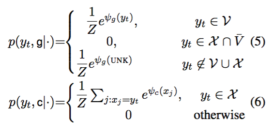
生成模式和拷贝模式的打分机制不同，分别为：

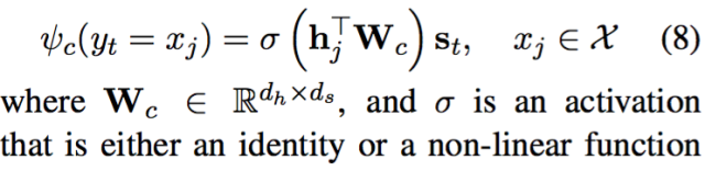
并且对Decoder部分的生成机制加了一个触发条件，这也是这篇论文的核心创新点，也即：

如果上一个Decoder的输出出现在了Source-text中，即源自于当前文本，则计算一个权重：

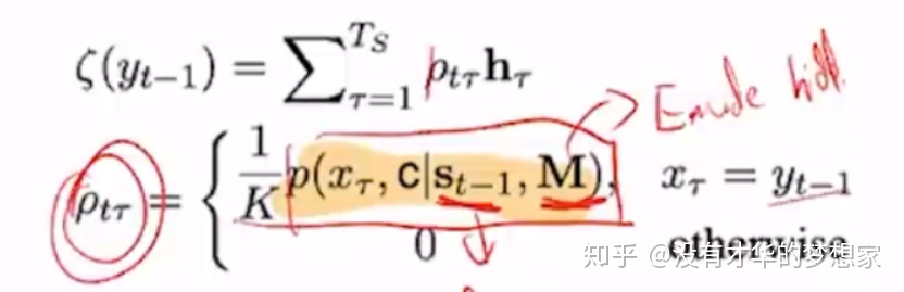
然后，在计算下一个Decoder的输出时，不仅仅要考虑上一个输出，如“Tony”，还需要再拼接一个加权平均，这个加权平均的计算公式如上，需要再考虑source文本的信息

即根据这个词分布的情况人为的规定（与上一篇文章的最大的区别，不是动态调整）应该来自于哪个概率，并且根据触发条件计算一个新的加权向量

3、文本生成任务的评价指标BLEU与Rouge

在机器翻译和文本生成这一块，BLEU（2002）和ROUGE（2003）是两种最为常见的评估指标，下面分别介绍

（1）BLEU

BLEU 的全称是 Bilingual evaluation understudy，BLEU 的分数取值范围是 0～1，分数越接近1，说明翻译的质量越高。BLEU 主要是基于精确率(Precision)的，下面是 BLEU 的整体公式。

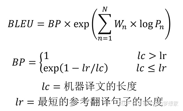
BLEU需要计算模型在n-gram下的精确度，公式中的Pn指的就是在n-gram下的精确度

BP是一个惩罚因子，主要针对的是Seq2Seq倾向于生成短句的问题，因此做了这样一个短句惩罚

根据语义的相关特性我们可以得出这样一个结论：BLEU的1-gram表示的是模型翻译终于原文的程度，而其他的n-gram表示的是翻译的流畅程度

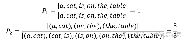
关于计算n-gram的方式可以参考这个例子：

机器翻译生成的译文: a cat is on the table

参考译文Reference: there is a cat on the table

若计算2-gram，则需要统计所有机器翻译的2-gram对出现在参考译文中的概率，也即：

但是这样的计算方式在一些场景下显然会有问题，尤其是机器翻译出现大量重复的场景下，如：

机器翻译生成的译文C: there there there there there

参考译文S:there is a cat on the table

这样的1-gram计算出来是1，显然是不对的，因此常常对BLEU的n-gram进行修正，公式如下：

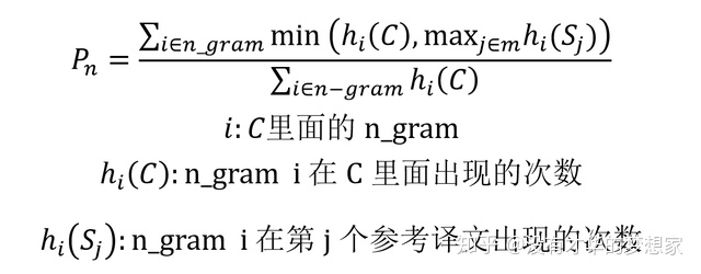
修正后的公式中的Pn：分母就是机器翻译语句的长度，

分子就是统计切分后的n-gram在机器翻译语句中的次数num1和在单一参考翻译语句中的出现最大次数num2的较小值，即min（num1,num2）

（2）Rouge

ROUGE 指标的全称是 (Recall-Oriented Understudy for Gisting Evaluation)，主要是基于召回率 (recall) 的。主要有四种计算方法：

ROUGE-N: 在 N-gram 上计算召回率

ROUGE-L: 考虑了机器译文和参考译文之间的最长公共子序列

ROUGE-W: 改进了ROUGE-L，用加权的方法计算最长公共子序列

ROUGE-S：对N-gram进行改进，但允许跳词，即允许不连续出现

本次项目主要用到的评价指标是ROUGE1、ROUGE2和ROUGE-L

ROUGE-N的计算公式为：统计 N-gram 上的召回率

分母是统计在参考译文中 N-gram 的个数，而分子是统计参考译文与机器译文共有的 N-gram 个数。

举例来说，

C: a cat is on the table

S1: there is a cat on the table

这个例子的ROUGE-1和ROUGE-2的分数如下：

ROUGE-L的计算公式则考虑了机器译文和参考译文的最长公共子序列，具体的计算公式为：

公式中的 RLCS 表示召回率，而 PLCS 表示精确率，FLCS 就是 ROUGE-L。

一般 beta 会设置为很大的数，因此 FLCS 几乎只考虑了 RLCS (即召回率)。

ROUGE-N的优缺点：

• 优点：直观、简洁、能反映次序
• 缺点：区分度不高，且当N>3时，ROUGE-N值通常很小。
• 应用场景：小文本摘要

ROUGE-L的优缺点

• 优点：不要求词的连续匹配，只要求按词的出现顺序匹配即可，能够像n-gram一样
• 优点：自动匹配最长公共子序列，不需要预先定义n-gram的长度。
• 优点：反映句子级的词序。
• 缺点：只计算一个最长子序列，最终的值忽略了其他备选的最长子序列及较短子序列的影响。
• 应用场景：单文本摘要

4、文本输出方法Beam-Search

同为Seq2Seq的文本输出方法，主要就是两种：Greedy Search和Beam Search，而Greedy Search其实就是设置Beam Size为1情况下的Beam Search

（1）Greedy Search

不管是哪种方式其实要解决的是同一个问题，即在Decoder得出概率分布之后，怎么根据概率选择单词

第一种也是最为直观的方式就是贪心法的思想，每次选取概率最大的

这种方式也就是Greedy Search

这种方式实际上考虑的是每一步的最优解，而不是全局的最优解，而且也没有办法证明这种办法能够取得全局最优

（2）Beam Search

由此衍生出了第二个方法，即Beam Search，Beam是桶的意思，Beam Size是桶中元素的个数

算法的基本思想就是每次保留所有概率中的TopK个，之后以这TopK个输出作为下一个time step的输入，再次得到输出，并在所有的结果中取TopK个，一定要注意这里是对所有的结果选取，不然就会导致可能的结果成指数型增长。

这里有一个地方需要注意：通常情况下我们用log对数来表示概率的累乘，从而在选取TopK个时比较方便，而根据概率的累乘性质我们知道，在这样的条件下模型会倾向于生成短一些的句子，也就是尽快的输出句子结束标志EOS，这个问题的解决办法是在预测时引入短句惩罚，具体做法后面会讲。

最后，Beam Search常使用堆栈来实现。

Beam Search概率累加图

5、模型训练优化Trick

这一部分主要是介绍模型在训练过程中运用的优化，可能跟第6点没有清晰的逻辑分割，算了，想到哪整理到哪吧

（1）Scheduled Sampling

在纯Seq2Seq的训练过程中，时常会发现模型的拟合效果欠佳，有时候生成的文本“胡言乱语”，Scheduled Sampling就是对其中一个原因提出的改进。

具体说来，在Decoder的训练阶段，我们在每一个time step输入的是目标样本，也即其实我们是将“答案”输了进去

而在测试和验证阶段，Decoder的每一步的输入是自身上一步的输出hidden state，也即“看不到答案”的，这就导致了偏差，即训练和预测的场景不同

而在预测的时候，如果上一个单词预测错误，还会产生多米诺骨牌效应，使后续的预测都出错

因此Scheduled Sampling的提出就是为了解决这个问题：

具体来说，在训练阶段，Decoder部分每一步的输入不单纯是目标样本，而是用一个超参数概率P，每一步以P的概率选择模型自身的输出作为下一步预测的输入，而1-P的概率选择目标文本，也即答案作为输入

一开始训练不充分，先让P小一些，尽量使用真实的文本作为输入（也称之为Teaching-Forcing），以达到快速拟合的目的。随着训练的进行，将P增大，多采用自身的输出作为下一个预测的输入，以增强模型的泛化能力。

随着训练的进行，P越来越大大，train-decoder模型最终变来和inference-decoder预测模型一样，消除了train-decoder与inference-decoder之间的差异

（2）Weight Tying

即共享Encoder和Decoder的embedding权重矩阵，使得其输入的词向量表达具有一致性

6、数据增强Trick

缺乏高质量的标注样本数据应该是NLP老生常谈的话题了，也为此对于数据量不是很大的场景，我们尝试使用一些数据增强的方式来进行优化

（1）单词替换

一个直观的想法是：如果我们将文本中的部分单词替换成语义相近的词，则可以得到一些新的并且合理的样本，从而丰富样本数据集。

但是，由于中文不像英文中有 WordNet 这种成熟的近义词词典可以使用，我们的具体做法是选择在 embedding 的词向量空间中寻找语义最接近的词。

通过使用在大量数据上预训练好的中文词向量，我们可以到每个词在该词向量空间中语义最接近的词，然后替换原始样本中的词，得到新的样本。

但是有一个问题是，如果我们替换了样本中的核心词汇，比如将文案中的体现关键卖点的词给替换掉了，可能会导致核心语义的丢失。对此，我们有两种解决办法：

1、通过 tfidf 权重对词表里的词进行排序，然后替换排序靠后的词

2、先通过无监督的方式挖掘样本中的主题词，然后只替换不属于主题词的词汇。

（2）回译

我们可以使用成熟的机器翻译模型，将中文文本翻译成一种外文，然后再翻译回中文，由此可以得到语义近似的新样本。

具体的说，就是通过调用一些成熟的机器翻译api，将文本进行多语言回译，从而扩充样本

（3）Bootstrapping

即自助生成样本。具体做法是利用训练好的模型对训练样本进行预测，生成新的样本，并将这部分样本并入原来的训练数据中，实现扩充数据的目的。

7、输出存在的问题与优化方法

这部分主要是分为两个部分：一个部分是阐述ACL2017那篇文章中用到的Coverage机制及fine-tune过程，另一部分是讲述针对输出存在的问题Beam Search中引入的一些优化

（1）Coverage机制

这部分是论文中所提到的Coverage机制，与下面要说到的Beam Search优化中的Coverage Normalization实现方式不同

重复问题几乎是所有生成模型的通病，作者提出的这个Coverage机制也着重是要解决这个问题

具体说来，在预测过程中，维护一个Coverage Vector：

这个向量是过去所有预测步计算的Attention分布的累加和，记录着模型已经关注过原文的哪些词,并且让这个coverage向量影响当前步的Attention计算

这样做的目的在于，在模型进行当前步attention计算的时候，告诉它之前它已经关注过的词，希望避免出现连续attention到某几个词上的情形。其中W_c是一个可学习的参数，具有和向量 v 一样的长度。

同时，coverage模型还添加一个额外的coverage loss，来对重复的attention作惩罚。

值得注意的是这个loss只会对重复的attention产生惩罚(min)，并不会强制要求模型关注原文中的每一个词。

最终，模型的整体损失函数为

这里的λ也是一个需要学习的超参数

（2）fine-tuning

这是作者在论文中提到的一个Trick：即训练该模型最好的方式是先不加coverage机制训练得到一个收敛的模型，然后加上coverage机制对该模型进行fine-tuning，因此可以定义两次训练，对第一次不加coverage机制的模型在训练后进行保存

而在fine-tuning的阶段，则将与Coverage机制无关的权重都固定，只训练与Coverage有关的权重

（3）Beam Search优化

这一部分主要是参考了OpenNMT中对于Beam-Search提出的优化方式，具体来说是三个Normalization：

1、Length Normalization

我们在Beam Search中提到的模型会倾向于生成短句的不足，可以通过对长度的归一化来解决

摘自OpenNMT对于Length Normalization的描述

2、Coverage Normalization

这里也是为了解决输出单词重复的问题，从而引入了这个Coverage作为惩罚项Penalty

目的是让 Decoder 均匀地关注于输入序列 x 的每一个 token，防止一些 token 获得过多的 Attention。

P_i,j表示的是第j个target对应第i个输入的Attention值，两个求和可以理解对输入某个单词在输出部分所有用到这个单词的Attention的累加

将这两个Normalization结合，可以得到新的得分函数：

3、EOS normalization：

为了解决 Beam Search 在 decode 的时候总是不会主动生成 token 的问题。加入对 EOS token 的概率的normalization。

其中∣ X ∣是source的长度，∣ Y ∣是当前target的长度，那么由上式可知，target长度越长的话，上述得分越低，这样就会防止出现生成一直不停止的情况

三、代码实现

这部分主要是对上述提到的模型和优化方法进行代码实现，我会划分成模块来放关键的代码，但不会展示所有的代码（主要是数据增强部分），完整的代码可以参见链接里的一位大佬的GitHub，请自行领取~

1、定义一个DataLoader来处理训练样本，实现包括字典的构建、token的索引以及 batch 的划分等功能

（1）通过预览原始数据json文件，我们可以看到数据格式大致是这样一个格式：

（2）转换json文件格式

按格式、类别读入文本数据

samples = set()
# Read json file.
json_path = os.path.join(abs_path, '../files/服饰_50k.json')
with open(json_path, 'r', encoding='utf8') as file:
    jsf = json.load(file)

for jsobj in jsf.values():
    title = jsobj['title'] + ' '  # Get title.
    kb = dict(jsobj['kb']).items()  # Get attributes.
    kb_merged = ''
    for key, val in kb:
        kb_merged += key+' '+val+' '  # Merge attributes.

    ocr = ' '.join(list(jieba.cut(jsobj['ocr'])))  # Get OCR text.
    texts = []
    texts.append(title + ocr + kb_merged)  # Merge them.
    reference = ' '.join(list(jieba.cut(jsobj['reference'])))
    for text in texts:
        sample = text+'<sep>'+reference  # Seperate source and reference.
        samples.add(sample)
write_path = os.path.join(abs_path, '../files/samples.txt')
write_samples(samples, write_path)

（3）词典处理

add_words函数：向词典⾥加⼊⼀个新词，需要完成对word2index、index2word和word2count三个变量的更新。

def add_words(self, words):
        """Add a new token to the vocab and do mapping between word and index.

        Args:
            words (list): The list of tokens to be added.
        """
        for word in words:
            if word not in self.word2index:
                self.word2index[word] = len(self.index2word)
                self.index2word.append(word)
        self.word2count.update(words)

build_vocab函数：需要实现控制数据集词典的⼤⼩（从config.max_vocab_size）读取这⼀参数。我们这里使⽤python的collection模块中的Counter来做。

def build_vocab(self, embed_file: str = None) -> Vocab:
        """Build the vocabulary for the data set.

        Args:
            embed_file (str, optional):
            The file path of the pre-trained embedding word vector.
            Defaults to None.

        Returns:
            vocab.Vocab: The vocab object.
        """
        # word frequency
        word_counts = Counter()
        count_words(word_counts,
                    [src + tgr for src, tgr in self.pairs])
        vocab = Vocab()
        # Filter the vocabulary by keeping only the top k tokens in terms of
        # word frequncy in the data set, where k is the maximum vocab size set
        # in "config.py".
        for word, count in word_counts.most_common(config.max_vocab_size):
            vocab.add_words([word])
        if embed_file is not None:
            count = vocab.load_embeddings(embed_file)
            print("%d pre-trained embeddings loaded." % count)

        return vocab

（4）自定义数据集SampleDataSet类：getitem函数是根据index取单词这里面的source2id涉及到了OOV单词的处理

class SampleDataset(Dataset):
    """The class represents a sample set for training.

    """
    def __init__(self, data_pair, vocab):
        self.src_sents = [x[0] for x in data_pair]
        self.trg_sents = [x[1] for x in data_pair]
        self.vocab = vocab
        # Keep track of how many data points.
        self._len = len(data_pair)

    def __getitem__(self, index):
        x, oov = source2ids(self.src_sents[index], self.vocab)
        return {
            'x': [self.vocab.SOS] + x + [self.vocab.EOS],
            'OOV': oov,
            'len_OOV': len(oov),
            'y': [self.vocab.SOS] +
            abstract2ids(self.trg_sents[index],
                         self.vocab, oov) + [self.vocab.EOS],
            'x_len': len(self.src_sents[index]),
            'y_len': len(self.trg_sents[index])
        }

    def __len__(self):
        return self._len

具体来说，对于OOV单词，将其映射到词表的最末尾并编号表示，如词表大小为500，则OOV词汇编号为501、502...

def source2ids(source_words, vocab):
    """Map the source words to their ids and return a list of OOVs in the source.
    Args:
        source_words: list of words (strings)
        vocab: Vocabulary object
    Returns:
        ids:
        A list of word ids (integers); OOVs are represented by their temporary
        source OOV number. If the vocabulary size is 50k and the source has 3
        OOVs tokens, then these temporary OOV numbers will be 50000, 50001,
        50002.
    oovs:
        A list of the OOV words in the source (strings), in the order
        corresponding to their temporary source OOV numbers.
    """
    ids = []
    oovs = []
    unk_id = vocab.UNK
    for w in source_words:
        i = vocab[w]
        if i == unk_id:  # If w is OOV
            if w not in oovs:  # Add to list of OOVs
                oovs.append(w)
            # This is 0 for the first source OOV, 1 for the second source OOV
            oov_num = oovs.index(w)
            # This is e.g. 20000 for the first source OOV, 50001 for the second
            ids.append(vocab.size() + oov_num)
        else:
            ids.append(i)
    return ids, oovs

对于reference文本，我们通过成abstract2ids函数将reference文本映射成Id。由于PGN可以⽣成在source⾥⾯出现过的OOV tokens，所以这次我们对reference的token ids需要换⼀种映射⽅式，即将在source里出现过的OOV tokens也记录下来并给⼀个临时的id，⽽不是直接替换为“”，以便在训练时计算损失更加准确。

具体说来是如下几行：

if w in source_oovs:  # If w is an in-source OOV
                # Map to its temporary source OOV number
                vocab_idx = vocab.size() + source_oovs.index(w)
                ids.append(vocab_idx)
def abstract2ids(abstract_words, vocab, source_oovs):
    """Map tokens in the abstract (reference) to ids.
       OOV tokens in the source will be remained.

    Args:
        abstract_words (list): Tokens in the reference.
        vocab (vocab.Vocab): The vocabulary.
        source_oovs (list): OOV tokens in the source.

    Returns:
        list: The reference with tokens mapped into ids.
    """
    ids = []
    unk_id = vocab.UNK
    for w in abstract_words:
        i = vocab[w]
        if i == unk_id:  # If w is an OOV word
            if w in source_oovs:  # If w is an in-source OOV
                # Map to its temporary source OOV number
                vocab_idx = vocab.size() + source_oovs.index(w)
                ids.append(vocab_idx)
            else:  # If w is an out-of-source OOV
                ids.append(unk_id)  # Map to the UNK token id
        else:
            ids.append(i)
    return ids

（5）生成DataLoader进行训练

Dataloader可以更方便的在数据集中取batch进行批训练，其中最重要的是collate_fn函数，它的作用是将数据集拆分为多个批，并对每个批进行填充；其中我们确定一个batch的最大长度，是根据sort_batch_by_len函数实现的

def collate_fn(batch):
    """Split data set into batches and do padding for each batch.

    Args:
        x_padded (Tensor): Padded source sequences.
        y_padded (Tensor): Padded reference sequences.
        x_len (int): Sequence length of the sources.
        y_len (int): Sequence length of the references.
        OOV (dict): Out-of-vocabulary tokens.
        len_OOV (int): Number of OOV tokens.
    """
    def padding(indice, max_length, pad_idx=0):
        pad_indice = [item + [pad_idx] * max(0, max_length - len(item))
                      for item in indice]
        return torch.tensor(pad_indice)

    data_batch = sort_batch_by_len(batch)

    x = data_batch["x"]
    x_max_length = max([len(t) for t in x])
    y = data_batch["y"]
    y_max_length = max([len(t) for t in y])

    OOV = data_batch["OOV"]
    len_OOV = torch.tensor(data_batch["len_OOV"])

    x_padded = padding(x, x_max_length)
    y_padded = padding(y, y_max_length)

    x_len = torch.tensor(data_batch["x_len"])
    y_len = torch.tensor(data_batch["y_len"])
    return x_padded, y_padded, x_len, y_len, OOV, len_OOV

2、实现模型baseline：Seq2Seq模型的训练模块

（1）Encoder部分

定义一个双向的LSTM作为Encoder部分

class Encoder(nn.Module):
    def __init__(self,vocab_size, embed_size, hidden_size, rnn_drop: float = 0):
        super(Encoder, self).__init__()
        self.embedding = nn.Embedding(vocab_size, embed_size)
        self.hidden_size = hidden_size
        self.lstm = nn.LSTM(embed_size,
                            hidden_size,
                            bidirectional=True,
                            dropout=rnn_drop,
                            batch_first=True)
    def forward(self, x):
        """Define forward propagation for the endoer.
        """
        embedded = self.embedding(x)
        output, hidden = self.lstm(embedded)
        return output, hidden

（2）Decoder部分

由一个单向的LSTM和两个线性层构成，前向传播的公式是论文中的式（4）

class Decoder(nn.Module):
    def __init__(self, vocab_size, embed_size, hidden_size, enc_hidden_size=None, is_cuda=True):
        super(Decoder, self).__init__()
        self.embedding = nn.Embedding(vocab_size, embed_size)
        self.DEVICE = torch.device('cuda') if is_cuda else torch.device('cpu')
        self.vocab_size = vocab_size
        self.hidden_size = hidden_size
        self.lstm = nn.LSTM(embed_size, hidden_size, batch_first=True)
        self.W1 = nn.Linear(self.hidden_size * 3, self.hidden_size)
        self.W2 = nn.Linear(self.hidden_size, vocab_size)

    def forward(self, x_t, decoder_states, context_vector):
        """Define forward propagation for the decoder.
        """
        decoder_emb = self.embedding(x_t)
        decoder_output, decoder_states = self.lstm(decoder_emb, decoder_states)
        # concatenate context vector and decoder state
        decoder_output = decoder_output.view(-1, config.hidden_size)
        concat_vector = torch.cat([decoder_output, context_vector], dim=-1)
        # calculate vocabulary distribution
        FF1_out = self.W1(concat_vector)
        FF2_out = self.W2(FF1_out)
        p_vocab = F.softmax(FF2_out, dim=1)
        h_dec, c_dec = decoder_states
        s_t = torch.cat([h_dec, c_dec], dim=2)
        return p_vocab, decoder_states

（3）Attention部分

Attention的计算公式是论文中的式（1）和式（2）

由于训练过程中会对batch中的样本进⾏padding，对于进⾏了padding的输⼊我们需要把填充的位置的attention weights给过滤掉（padding mask），然后对剩下位置的attention weights进⾏归⼀化

根据论⽂中的公式(3)计算context vector

class Attention(nn.Module):
    def __init__(self, hidden_units):
        super(Attention, self).__init__()
        # Define feed-forward layers.
        self.Wh = nn.Linear(2*hidden_units, 2*hidden_units, bias=False)
        self.Ws = nn.Linear(2*hidden_units, 2*hidden_units)

    def forward(self,
                decoder_states,
                encoder_output,
                x_padding_masks,
                coverage_vector):
        """Define forward propagation for the attention network.
        """
        # Concatenate h and c to get s_t and expand the dim of s_t.
        h_dec, c_dec = decoder_states
        s_t = torch.cat([h_dec, c_dec], dim=2)
        s_t = s_t.transpose(0, 1)
        s_t = s_t.expand_as(encoder_output).contiguous()
        # calculate attention scores
        encoder_features = self.Wh(encoder_output.contiguous())
        decoder_features = self.Ws(s_t)
        att_inputs = encoder_features + decoder_features
        score = self.v(torch.tanh(att_inputs))
        attention_weights = F.softmax(score, dim=1).squeeze(2)
        attention_weights = attention_weights * x_padding_masks
        # Normalize attention weights after excluding padded positions.
        normalization_factor = attention_weights.sum(1, keepdim=True)
        attention_weights = attention_weights / normalization_factor
        context_vector = torch.bmm(attention_weights.unsqueeze(1),
                                   encoder_output)
        context_vector = context_vector.squeeze(1)
        return context_vector, attention_weights

（4）ReduceState模块：实现数据降维

由于Encoder部分选用的是双向LSTM，而Decoder部分选用的是单向LSTM，因此若直接对Encoder的hidden state与Decoder的hidden state进行运算势必会出现维度冲突，因此需要维度降维，这里采用的是简单的将Encoder的双向LSTM中两个方向的hidden state简单相加

class ReduceState(nn.Module):
    """
    Since the encoder has a bidirectional LSTM layer while the decoder has a
    unidirectional LSTM layer, we add this module to reduce the hidden states
    output by the encoder (merge two directions) before input the hidden states
    nto the decoder.
    """
    def __init__(self):
        super(ReduceState, self).__init__()

    def forward(self, hidden):
        """The forward propagation of reduce state module.

        Args:
            hidden (tuple):
                Hidden states of encoder,
                each with shape (2, batch_size, hidden_units).

        Returns:
            tuple:
                Reduced hidden states,
                each with shape (1, batch_size, hidden_units).
        """
        h, c = hidden
        h_reduced = torch.sum(h, dim=0, keepdim=True)
        c_reduced = torch.sum(c, dim=0, keepdim=True)
        return (h_reduced, c_reduced)

（5）Seq2Seq整体前向传导

• 对输⼊序列x进⾏处理，对于oov的token，需要将他们的index转换成 UNK token
• ⽣成输⼊序列x的padding mask
• 得到encoder的输出和隐状态，并对隐状态进⾏降维后作为decoder的初始隐状态
• 对于每⼀个time step，以输⼊序列y的y_t作为输⼊，y_t+1作为target，计算attention，然后⽤ decoder得到P_vocab，找到target对应的词在P_vocab中对应的概率target_probs，然后计算time step t的损失，最后加上padding mask，计算time step t损失的公式是论文中的式（6）

• 计算整个序列的平均loss，计算公式是论文中的式（7）

• 计算整个batch的平均loss并返回

class Seq2seq(nn.Module):
    def __init__(self, v):
        super(Seq2seq, self).__init__()
        self.v = v
        self.DEVICE = config.DEVICE
        self.attention = Attention(config.hidden_size)
        self.encoder = Encoder(len(v),config.embed_size,config.hidden_size,)
        self.decoder = Decoder(len(v),config.embed_size,config.hidden_size,)
        self.reduce_state = ReduceState()


    def forward(self, x, x_len, y, len_oovs, batch, num_batches):
        """Define the forward propagation for the model.
        """
        x_copy = replace_oovs(x, self.v)
        x_padding_masks = torch.ne(x, 0).byte().float()
        encoder_output, encoder_states = self.encoder(x_copy)
        # Reduce encoder hidden states.
        decoder_states = self.reduce_state(encoder_states)
        # Calculate loss for every step.
        step_losses = []
        for t in range(y.shape[1]-1):
            # Do teacher forcing.
            x_t = y[:, t]
            x_t = replace_oovs(x_t, self.v)
            y_t = y[:, t+1]
            # Get context vector from the attention network.
            context_vector, attention_weights = self.attention(decoder_states, encoder_output, x_padding_masks, coverage_vector)
            # Get vocab distribution and hidden states from the decoder.
            p_vocab, decoder_states= self.decoder(x_t.unsqueeze(1), decoder_states, context_vector)
            # Get the probabilities predict by the model for target tokens.
            y_t = replace_oovs(y_t, self.v)
            target_probs = torch.gather(p_vocab, 1, y_t.unsqueeze(1))
            target_probs = target_probs.squeeze(1)
            # Apply a mask such that pad zeros do not affect the loss
            mask = torch.ne(y_t, 0).byte()
            # Do smoothing to prevent getting NaN loss because of log(0).
            loss = -torch.log(target_probs + config.eps)
            mask = mask.float()
            loss = loss * mask
            step_losses.append(loss)

        sample_losses = torch.sum(torch.stack(step_losses, 1), 1)
        # get the non-padded length of each sequence in the batch
        seq_len_mask = torch.ne(y, 0).byte().float()
        batch_seq_len = torch.sum(seq_len_mask, dim=1)
        # get batch loss by dividing the loss of each batch
        # by the target sequence length and mean
        batch_loss = torch.mean(sample_losses / batch_seq_len)
        return batch_loss

3、实现模型优化：PGN网络+Coverage机制

（1）Encoder部分没有变化

（2）Decoder部分：

• 定义一个线性层w_gen
• 实现P_gen的计算，公式是论文中的公式（8）

self.w_gen = nn.Linear(self.hidden_size * 4 + embed_size, 1)
p_gen = torch.sigmoid(self.w_gen(x_gen))
def forward(self, x_t, decoder_states, context_vector):
        """Define forward propagation for the decoder.
        """
        decoder_emb = self.embedding(x_t)
        decoder_output, decoder_states = self.lstm(decoder_emb, decoder_states)
        # concatenate context vector and decoder state
        decoder_output = decoder_output.view(-1, config.hidden_size)
        concat_vector = torch.cat(
            [decoder_output,
             context_vector],
            dim=-1)
        # calculate vocabulary distribution
        FF1_out = self.W1(concat_vector)
        FF2_out = self.W2(FF1_out)
        p_vocab = F.softmax(FF2_out, dim=1)
        h_dec, c_dec = decoder_states
        s_t = torch.cat([h_dec, c_dec], dim=2)
        p_gen = None
        if config.pointer:
            # Calculate p_gen.
            x_gen = torch.cat([context_vector,s_t.squeeze(0),decoder_emb.squeeze(1)], dim=-1)
            p_gen = torch.sigmoid(self.w_gen(x_gen))
        return p_vocab, decoder_states, p_gen

（3）Attention机制：

• 在计算Attention weight时加入了Coverage Vector，见公式（11）

• 并对Coverage Vector进行更新，见公式（10）

定义W_c线性层：

self.wc = nn.Linear(1, 2*hidden_units, bias=False)

定义W_c的前向传播计算：

if config.coverage:
            coverage_features = self.wc(coverage_vector.unsqueeze(2))  # wc c
            att_inputs = att_inputs + coverage_features

定义Coverage Vector的更新（其实就是累加）：

if config.coverage:
            coverage_vector = coverage_vector + attention_weights
def forward(self, decoder_states, encoder_output, x_padding_masks, coverage_vector):
        """Define forward propagation for the attention network.
        """
        # Concatenate h and c to get s_t and expand the dim of s_t.
        h_dec, c_dec = decoder_states
        s_t = torch.cat([h_dec, c_dec], dim=2)
        s_t = s_t.transpose(0, 1)
        s_t = s_t.expand_as(encoder_output).contiguous()
        # calculate attention scores
        encoder_features = self.Wh(encoder_output.contiguous())
        decoder_features = self.Ws(s_t)
        att_inputs = encoder_features + decoder_features
        # Add coverage feature.
        if config.coverage:
            coverage_features = self.wc(coverage_vector.unsqueeze(2))  # wc c
            att_inputs = att_inputs + coverage_features
        score = self.v(torch.tanh(att_inputs))
        attention_weights = F.softmax(score, dim=1).squeeze(2)
        attention_weights = attention_weights * x_padding_masks

        # Normalize attention weights after excluding padded positions.
        normalization_factor = attention_weights.sum(1, keepdim=True)
        attention_weights = attention_weights / normalization_factor       
        context_vector = torch.bmm(attention_weights.unsqueeze(1), encoder_output)
        context_vector = context_vector.squeeze(1)
        # Update coverage vector.
        if config.coverage:
            coverage_vector = coverage_vector + attention_weights
        return context_vector, attention_weights, coverage_vector

（4）ReduceState模块：实现数据降维

这部分没有变化

（5）get_final_distribution函数

这一部分得到总体的预测概率分布图：

具体的实现方法为：先对 P_vocab 进⾏扩展，将 source 中的 oov 添 加到 P_vocab 的尾部，得到P_vocab_extend 这样 attention weights 中的每⼀个 token 都能在 P_vocab_extend 中找到对应的位置，然后 将对应的 attention weights 叠加到扩展后的 P_vocab_extend 中的对 应位置，得到 final distribution。

def get_final_distribution(self, x, p_gen, p_vocab, attention_weights, max_oov):
        """Calculate the final distribution for the model.
        """
        batch_size = x.size()[0]
        # Clip the probabilities.
        p_gen = torch.clamp(p_gen, 0.001, 0.999)
        # Get the weighted probabilities.
        p_vocab_weighted = p_gen * p_vocab
        attention_weighted = (1 - p_gen) * attention_weights

        # Get the extended-vocab probability distribution    
        extension = torch.zeros((batch_size, max_oov)).float().to(self.DEVICE)
        p_vocab_extended = torch.cat([p_vocab_weighted, extension], dim=1)
        # Add the attention weights to the corresponding vocab positions.
        final_distribution =  p_vocab_extended.scatter_add_(dim=1, index=x, src=attention_weighted)
        return final_distribution

（6）PGN网络整体的forward

与Seq2Seq相比多了一个计算Coverage Loss的过程，计算公式是论文中的公式（12）和公式（13）

loss函数的前半部分是Seq2Seq模型的loss，后半部分是Coverage Loss

其中式（12）的实现代码：

# Add coverage loss.
            ct_min = torch.min(attention_weights, coverage_vector)
            cov_loss = torch.sum(ct_min, dim=1)
            loss = loss + config.LAMBDA * cov_loss
def forward(self, x, x_len, y, len_oovs, batch, num_batches):
        """Define the forward propagation for the model.
        """
        x_copy = replace_oovs(x, self.v)
        x_padding_masks = torch.ne(x, 0).byte().float()
        encoder_output, encoder_states = self.encoder(x_copy)
        # Reduce encoder hidden states.
        decoder_states = self.reduce_state(encoder_states)
        # Initialize coverage vector.
        coverage_vector = torch.zeros(x.size()).to(self.DEVICE)
        # Calculate loss for every step.
        step_losses = []
        for t in range(y.shape[1]-1):
            # Do teacher forcing.
            x_t = y[:, t]
            x_t = replace_oovs(x_t, self.v)

            y_t = y[:, t+1]
            # Get context vector from the attention network.
            context_vector, attention_weights, next_coverage_vector = 
                self.attention(decoder_states,
                               encoder_output,
                               x_padding_masks,
                               coverage_vector)
            # Get vocab distribution and hidden states from the decoder.
            p_vocab, decoder_states, p_gen = self.decoder(x_t.unsqueeze(1),
                                                          decoder_states,
                                                          context_vector)

            final_dist = self.get_final_distribution(x,
                                                     p_gen,
                                                     p_vocab,
                                                     attention_weights,
                                                     torch.max(len_oovs))

            # Get the probabilities predict by the model for target tokens.
            target_probs = torch.gather(final_dist, 1, y_t.unsqueeze(1))
            target_probs = target_probs.squeeze(1)

            # Apply a mask such that pad zeros do not affect the loss
            mask = torch.ne(y_t, 0).byte()
            # Do smoothing to prevent getting NaN loss because of log(0).
            loss = -torch.log(target_probs + config.eps)

            # Add coverage loss.
            ct_min = torch.min(attention_weights, coverage_vector)
            cov_loss = torch.sum(ct_min, dim=1)
            loss = loss + config.LAMBDA * cov_loss
            coverage_vector = next_coverage_vector

            mask = mask.float()
            loss = loss * mask
            step_losses.append(loss)

        sample_losses = torch.sum(torch.stack(step_losses, 1), 1)
        # get the non-padded length of each sequence in the batch
        seq_len_mask = torch.ne(y, 0).byte().float()
        batch_seq_len = torch.sum(seq_len_mask, dim=1)

        # get batch loss by dividing the target sequence length and mean
        batch_loss = torch.mean(sample_losses / batch_seq_len)
        return batch_loss

4、模型解码

（1）实现Greedy Search

贪心思想，argmax每个输出概率得到单词即可

x_t = torch.argmax(final_dist, dim=1).to(self.DEVICE)
def greedy_search(self,
                      x,
                      max_sum_len,
                      len_oovs,
                      x_padding_masks):
        """Function which returns a summary by always picking
        """

        # Get encoder output and states.
        encoder_output, encoder_states = self.model.encoder(
            replace_oovs(x, self.vocab))

        # Initialize decoder's hidden states with encoder's hidden states.
        decoder_states = self.model.reduce_state(encoder_states)

        # Initialize decoder's input at time step 0 with the SOS token.
        x_t = torch.ones(1) * self.vocab.SOS
        x_t = x_t.to(self.DEVICE, dtype=torch.int64)
        summary = [self.vocab.SOS]
        coverage_vector = torch.zeros((1, x.shape[1])).to(self.DEVICE)
        # Generate hypothesis with maximum decode step.
        while int(x_t.item()) != (self.vocab.EOS) 
                and len(summary) < max_sum_len:
            context_vector, attention_weights, coverage_vector = 
                self.model.attention(decoder_states,
                                     encoder_output,
                                     x_padding_masks,
                                     coverage_vector)
            p_vocab, decoder_states, p_gen = 
                self.model.decoder(x_t.unsqueeze(1),
                                   decoder_states,
                                   context_vector)
            final_dist = self.model.get_final_distribution(x,
                                                           p_gen,
                                                           p_vocab,
                                                           attention_weights,
                                                           torch.max(len_oovs))
            # Get next token with maximum probability.
            x_t = torch.argmax(final_dist, dim=1).to(self.DEVICE)
            decoder_word_idx = x_t.item()
            summary.append(decoder_word_idx)
            x_t = replace_oovs(x_t, self.vocab)
        return summary

（2）Beam Search及优化

优化主要指的是加入了Length normalization， Coverage normalization以及End of sentence normalization

首先，首先定义一个 Beam 类，作为一个存放候选序列的容器，属性需维护当前序列中的 token 以及对应的对数概率，同时还需维护跟当前 timestep 的 Decoder 相关的一些变量。此外，还需要给 Beam 类实现两个函数：一个 extend 函数用以扩展当前的序列（即添加新的 time step的 token 及相关变量）；一个 score 函数用来计算当前序列的分数（在Beam类下的seq_score函数中有Length normalization以及Coverage normalization）

class Beam(object):
    def __init__(self,
                 tokens,
                 log_probs,
                 decoder_states,
                 coverage_vector):
        self.tokens = tokens
        self.log_probs = log_probs
        self.decoder_states = decoder_states
        self.coverage_vector = coverage_vector

    def extend(self,
               token,
               log_prob,
               decoder_states,
               coverage_vector):
        return Beam(tokens=self.tokens + [token],
                    log_probs=self.log_probs + [log_prob],
                    decoder_states=decoder_states,
                    coverage_vector=coverage_vector)
    def seq_score(self):
        """
        This function calculate the score of the current sequence.
        """
        len_Y = len(self.tokens)
        # Lenth normalization
        ln = (5+len_Y)**config.alpha / (5+1)**config.alpha
        cn = config.beta * torch.sum(  # Coverage normalization
            torch.log(
                config.eps +
                torch.where(
                    self.coverage_vector < 1.0,
                    self.coverage_vector,
                    torch.ones((1, self.coverage_vector.shape[1])).to(torch.device(config.DEVICE))
                )
            )
        )
        score = sum(self.log_probs) / ln + cn
        return score

接着我们需要实现一个 best_k 函数，作用是将一个 Beam 容器中当前 time step 的变量传入 Decoder 中，计算出新一轮的词表概率分布，并从中选出概率最大的 k 个 token 来扩展当前序列（其中加入了End of sentence normalization），得到 k 个新的候选序列。

def best_k(self, beam, k, encoder_output, x_padding_masks, x, len_oovs):
        """Get best k tokens to extend the current sequence at the current time step.
        """
        # use decoder to generate vocab distribution for the next token
        x_t = torch.tensor(beam.tokens[-1]).reshape(1, 1)
        x_t = x_t.to(self.DEVICE)

        # Get context vector from attention network.
        context_vector, attention_weights, coverage_vector = 
            self.model.attention(beam.decoder_states,
                                 encoder_output,
                                 x_padding_masks,
                                 beam.coverage_vector)
、
        p_vocab, decoder_states, p_gen = 
            self.model.decoder(replace_oovs(x_t, self.vocab),
                               beam.decoder_states,
                               context_vector)

        final_dist = self.model.get_final_distribution(x,
                                                       p_gen,
                                                       p_vocab,
                                                       attention_weights,
                                                       torch.max(len_oovs))
        # Calculate log probabilities.
        log_probs = torch.log(final_dist.squeeze())
        # EOS token penalty. Follow the definition in
        log_probs[self.vocab.EOS] *= 
            config.gamma * x.size()[1] / len(beam.tokens)
        log_probs[self.vocab.UNK] = -float('inf')
        # Get top k tokens and the corresponding logprob.
        topk_probs, topk_idx = torch.topk(log_probs, k)
        best_k = [beam.extend(x,
                  log_probs[x],
                  decoder_states,
                  coverage_vector) for x in topk_idx.tolist()]
        return best_k

最后我们实现主函数 beam_search。初始化encoder、attention和decoder的输⼊，然后对于每⼀个decoder time step，对于现有的k个beam，我们分别利⽤best_k函数来得到各⾃最佳的k个extended beam，也就是每个decode step我们会得到k个新的beam，然后只保留分数最⾼的k个，作为下⼀轮需要扩展的k个beam。为了只保留分数最⾼的k个beam，我们可以⽤⼀个堆(heap)来实现，堆的中只保存k个节点，根结点保存分数最低的beam

def beam_search(self,
                    x,
                    max_sum_len,
                    beam_width,
                    len_oovs,
                    x_padding_masks):
        """Using beam search to generate summary.
        """
        # run body_sequence input through encoder
        encoder_output, encoder_states = self.model.encoder(
            replace_oovs(x, self.vocab))
        coverage_vector = torch.zeros((1, x.shape[1])).to(self.DEVICE)
        # initialize decoder states with encoder forward states
        decoder_states = self.model.reduce_state(encoder_states)
        # initialize the hypothesis with a class Beam instance.
        init_beam = Beam([self.vocab.SOS],
                         [0],
                         decoder_states,
                         coverage_vector)
        k = beam_width
        curr, completed = [init_beam], []
        # use beam search for max_sum_len (maximum length) steps
        for _ in range(max_sum_len):
            # get k best hypothesis when adding a new token
            topk = []
            for beam in curr:
                # When an EOS token is generated, add the hypo to the completed
                if beam.tokens[-1] == self.vocab.EOS:
                    completed.append(beam)
                    k -= 1
                    continue
                for can in self.best_k(beam,
                                       k,
                                       encoder_output,
                                       x_padding_masks,
                                       x,
                                       torch.max(len_oovs)
                                       ):
                    # Using topk as a heap to keep track of top k candidates.
                    add2heap(topk, (can.seq_score(), id(can), can), k)

            curr = [items[2] for items in topk]
            # stop when there are enough completed hypothesis
            if len(completed) == beam_width:
                break
        completed += curr
        # sort the hypothesis by normalized probability and choose the best one
        result = sorted(completed,
                        key=lambda x: x.seq_score(),
                        reverse=True)[0].tokens
        return result

5、ROUGE评估

本次项目中主要使用的评估指标是ROUGE-1、ROUGE-2以及ROUGE-L

rouge直接调用库函数来做，并没有手动实现：

class RougeEval():
    def __init__(self, path):
        self.path = path
        self.scores = None
        self.rouge = Rouge()
        self.sources = []
        self.hypos = []
        self.refs = []
        self.process()
    def process(self):
        print('Reading from ', self.path)
        with open(self.path, 'r') as test:
            for line in test:
                source, ref = line.strip().split('<sep>')
                ref = ''.join(list(jieba.cut(ref))).replace('。', '.')
                self.sources.append(source)
                self.refs.append(ref)
        print(f'Test set contains {len(self.sources)} samples.')


    def build_hypos(self, predict):
        print('Building hypotheses.') 
        count = 0
        for source in self.sources:
            count += 1
            if count % 100 == 0:
                print(count)
            self.hypos.append(predict.predict(source.split()))

    def get_average(self):
        assert len(self.hypos) > 0, 'Build hypotheses first!'
        print('Calculating average rouge scores.')
        return self.rouge.get_scores(self.hypos, self.refs, avg=True)

    def one_sample(self, hypo, ref):
        return self.rouge.get_scores(hypo, ref)[0]
rouge_eval = RougeEval(config.test_data_path)
predict = Predict()
rouge_eval.build_hypos(predict)
result = rouge_eval.get_average()
print('rouge1: ', result['rouge-1'])
print('rouge2: ', result['rouge-2'])
print('rougeL: ', result['rouge-l'])

6、模型优化技巧

（1）Weight Tying

即共享 Encoder 和 Decoder 的 embedding 权重矩阵，使得其输入的词向量表达具有一致性。

这里使用的是使⽤的是three-way tying，即Encoder的input embedding，Decoder的input emdedding和Decoder的output embedding之间的权重共享

Encoder部分：

if config.weight_tying:
            embedded = decoder_embedding(x)
        else:
            embedded = self.embedding(x)

Decoder部分：

if config.weight_tying:
            FF2_out = torch.mm(FF1_out, torch.t(self.embedding.weight))
        else:
            FF2_out = self.W2(FF1_out)

（2）Scheduled sampling

理论部分已经讲过，就是按照一定的概率进行Teaching-forcing，而阈值概率我们让他随机产生，而是否进行Scheduled Sampling的概率与训练的epoch数或者batch数控制

class ScheduledSampler():
    def __init__(self, phases):
        self.phases = phases
        self.scheduled_probs = [i / (self.phases - 1) for i in range(self.phases)]

    def teacher_forcing(self, phase):
        """According to a certain probability to choose whether to execute teacher_forcing
        """
        sampling_prob = random.random()
        if sampling_prob >= self.scheduled_probs[phase]:
            return True
        else:
            return False

四、结果与思考

由于设备原因，我只跑了部分模型，包括最基本的Seq2Seq以及加入部分优化Trick的模型，这里贴的是链接里大佬们跑出来的结果，当然都比不上原论文作者，毕竟人家的数据集无论是数量还是质量上都远胜于我

至于Coverage机制与其欲解决的问题，只能说在实验结果以及原理上确实做到了对原有模型的改进。Coverage机制从Attention这一根源一定程度的限制了词语重复的出现，并用loss的方式强制让模型在训练中学会优化这个问题，可以说无论是想法还是实现效果都是非常好的。但是否完全解决了词语重复的问题，我觉得是并没有的，因为按照这个方法，更多的应该是对模型起到了一种比较好的限制作用。

五、Reference文档和博客

将本文主要参考的资料文档博客链接陈列如下：

1、

PaperWeekly：Incorporating Copying Mechanism in Sequence-to-Sequence Learning​zhuanlan.zhihu.com

2、

机器翻译与自动文摘评价指标 BLEU 和 ROUGE​baijiahao.baidu.com

3、

机器翻译评估指标之BLEU​www.jianshu.com

4、

seq2seq聊天模型（二）--Scheduled Sampling​www.cnblogs.com

5、

https://opennmt.net/OpenNMT/translation/beam_search/​opennmt.net

6、

论文阅读笔记《Get To The Point: Summarization with Pointer-Generator Networks》​blog.csdn.net

7、

https://github.com/mgh5212819/Chinese-Marketing-text-generation​github.com

8、

Beam search - OpenNMT​opennmt.net

9、

https://blog.csdn.net/qq_38556984/article/details/108294319​blog.csdn.net