【论文精读】FeCoGraph: Label-Aware Federated Graph Contrastive Learning for Few-Shot Network Intrusion Dec

FeCoGraph: Label-Aware Federated Graph Contrastive Learning for Few-Shot Network Intrusion Detection

FeCoGraph：用于少样本网络入侵检测的标签感知联邦图对比学习

Abstract-With increasing cyber attacks over the Internet, network intrusion detection systems (NIDS) have been an indispensable barrier to protecting network security. Taking advantage of automatically capturing topology connections, recent deep graph learning approaches have achieved remarkable performance in distinguishing different types of malicious flows. However, there remain some critical challenges. 1) previous supervised learning methods rely heavily on abundant and high-quality annotated samples, while label annotation requires abundant time and expert knowledge. 2) Centralized methods require all data to be uploaded to a server for learning behavior patterns, which results in high detection latency and critical privacy leakage. 3) Diverse attack scenarios exhibit highly imbalanced distribution, making it hard to characterize abnormal behaviors. To address these issues, we proposed FeCoGraph, a label-aware federated graph contrastive learning framework for intrusion detection in few-shot scenarios. The line graph is introduced to directly process flow embeddings, which are compatible with diverse GNNs. Furthermore, We formulate a graph contrastive learning task to effectively leverage label information, allowing intra-class embeddings more compact than inter-class embeddings. To improve the scalability of NIDS, we utilize federated learning to cover more attack scenarios while protecting data privacy. Experiment results show that FeCoGraph surpass E-graphSAGE with an average $8.36\%$ accuracy on binary classification and $6.77\%$ accuracy on multiclass classification,demonstrating the efficiency of our approach.

摘要 — 随着互联网上网络攻击的日益增多，网络入侵检测系统（NIDS）已成为保护网络安全不可或缺的屏障。利用自动捕获拓扑连接的优势，最近的深度图学习方法在区分不同类型的恶意流量方面取得了显著的性能。然而，仍然存在一些关键挑战。1）以前的监督学习方法严重依赖丰富且高质量的标注样本，而标签标注需要大量时间和专家知识。2）集中式方法要求将所有数据上传到服务器以学习行为模式，这导致检测延迟高和严重的隐私泄露。3）不同的攻击场景呈现出高度不平衡的分布，使得难以刻画异常行为。为了解决这些问题，我们提出了 FeCoGraph，这是一种用于少样本场景入侵检测的标签感知联邦图对比学习框架。引入线图直接处理流量嵌入，这些嵌入与各种图神经网络（GNN）兼容。此外，我们制定了一个图对比学习任务，以有效利用标签信息，使类内嵌入比类间嵌入更紧凑。为了提高 NIDS 的可扩展性，我们利用联邦学习在保护数据隐私的同时覆盖更多攻击场景。实验结果表明，FeCoGraph 在二分类上的平均准确率超过 E - graphSAGE $8.36\%$ ，在多分类上的准确率超过 $6.77\%$ ，证明了我们方法的有效性。

Index Terms-Network intrusion detection, few-shot learning, graph contrastive learning, graph neural networks.

索引术语 — 网络入侵检测、少样本学习、图对比学习、图神经网络。

I. INTRODUCTION

I. 引言

THE last few decades have witnessed an increasing number of cyberattacks towards Internet infrastructures around the world. Consequently, network intrusion detection systems (NIDS) have been an essential component in rapidly detecting emerging security threats. There are two kinds of methods, including signature-based [1] and anomaly-based methods [2]. While signature-based methods suffer from low detection rates and poor scalability, anomaly-based approaches have broader prospects with the potential to detect emerging and diverse attacks.

在过去的几十年里，针对全球互联网基础设施的网络攻击数量不断增加。因此，网络入侵检测系统（NIDS）已成为快速检测新兴安全威胁的重要组成部分。有两种方法，包括基于特征签名的方法 [1] 和基于异常的方法 [2] 。基于特征签名的方法存在检测率低和可扩展性差的问题，而基于异常的方法具有检测新兴和多样化攻击的潜力，前景更为广阔。

Previous studies have introduced deep learning methods to solve NIDS problems. High-level discriminative features are extracted from statistical features for classification. Although they have achieved excellent performance, they don’t consider the relation between network flows. Some advanced attacks launched by a cluster of computers, such as distributed denial-of-service (DDoS) attacks [3], can be depicted as host interactions. When we convert network traffic into a graph, these host interactions can be captured by graph neural networks (GNNs) to enhance the topology-aware expressive capabilities [4].

以往的研究引入了深度学习方法来解决 NIDS 问题。从统计特征中提取高级判别特征进行分类。虽然它们取得了优异的性能，但没有考虑网络流量之间的关系。一些由一组计算机发起的高级攻击，如分布式拒绝服务（DDoS）攻击 [3] ，可以描述为主机交互。当我们将网络流量转换为图时，这些主机交互可以被图神经网络（GNN）捕获，以增强拓扑感知表达能力 [4] 。

The last few years have seen an increased number of GNN-based solutions for network intrusion detection. Some studies proposed tailored GNN models for automatically detecting malicious botnet nodes [5], [6]. However, only the structural information is used. Regarding intrusion detection as an edge classification problem, E-GraphSAGE [7] reformulated Graph-SAGE to aggregate neighboring edge features. Chang et al. [8] incorporated the residual connection into E-GraphSAGE to tackle the imbalance issue. Other works are based on time-spatial analysis, with the time correlation-aware graph [9] or the interaction history [10]. The above methods are used as supervised models, requiring a huge amount of labeled data. However, annotating numerous labels is a time-consuming and labor-intensive task, hindering adaptation to unknown attacks.

在过去的几年里，基于 GNN 的网络入侵检测解决方案数量不断增加。一些研究提出了定制的 GNN 模型，用于自动检测恶意僵尸网络节点 [5] 、[6] 。然而，仅使用了结构信息。E - GraphSAGE [7] 将入侵检测视为边分类问题，重新构建了 Graph - SAGE 以聚合相邻边的特征。Chang 等人 [8] 将残差连接融入 E - GraphSAGE 以解决不平衡问题。其他工作基于时空分析，使用时间相关感知图 [9] 或交互历史 [10] 。上述方法均作为监督模型使用，需要大量的标注数据。然而，标注大量标签是一项耗时且费力的任务，阻碍了对未知攻击的适应。

Recent studies integrate self-supervised learning techniques into GNN models in the absence of labeled data. In Anomal-E [11], deep graph infomax objective [12] is leveraged to increase the amount of shared information between local and global representation. TS-IDS [13] enhances the expressive ability of edge embedding by predicting nodes’ properties based on the volume of traffic traversing them. Compared with Anomal-E, TS-IDS provides an end-to-end training paradigm, which obviates the need for selecting the pooling function [14] and optimizing the encoder and classifier separately.

最近的研究在没有标注数据的情况下将自监督学习技术集成到 GNN 模型中。在 Anomal - E [11] 中，利用深度图信息最大化目标 [12] 来增加局部和全局表示之间的共享信息量。TS - IDS [13] 通过基于流经节点的流量量预测节点属性来增强边嵌入的表达能力。与 Anomal - E 相比，TS - IDS 提供了一种端到端的训练范式，无需选择池化函数 [14] ，也无需分别优化编码器和分类器。

Although these two approaches have demonstrated considerable performance without requiring labeled data, they still encounter three critical challenges. First, recently attack behaviors usually exhibit intricate patterns, while limited network traffic samples are available. This might increase the difficulty of malicious network flow detection with restricted samples. Secondly, cyber attacks usually demonstrate imbalanced distribution and vague boundaries between different attack scenarios, making it hard to accurately characterize abnormal behavioral patterns. Considering long-term APT attacks as an example, the attackers can constantly adjust attack strategies until reaching their goal of extracting critical information, leading to the complexity and chronicity in extracting intrinsic features of such an attack. Finally, existing centralized NIDS approach will inevitably cause heavy computation overheads and high latency, thereby resulting in detection delay of abnormal behaviors and poor scalability in large-scale networks. Since network flow data are collected from different institutions, centralized data transmission and storage also heavily incurs privacy concerns [15]. Given the challenges brought by diverse emerging attacks, limited number of available samples and privacy concerns about distributed data, it is of great significance to develop an effective federated graph learning framework towards label-scarce NIDS scenario.

尽管这两种方法在无需标注数据的情况下展现出了相当不错的性能，但它们仍面临三个关键挑战。首先，近期的攻击行为通常呈现出复杂的模式，而可用的网络流量样本却有限。这可能会增加在样本受限的情况下检测恶意网络流量的难度。其次，网络攻击通常表现出分布不均衡的特点，且不同攻击场景之间的界限模糊，这使得准确刻画异常行为模式变得困难。以长期的高级持续性威胁（APT）攻击为例，攻击者可以不断调整攻击策略，直至达到提取关键信息的目标，这导致了提取此类攻击内在特征的复杂性和长期性。最后，现有的集中式网络入侵检测系统（NIDS）方法不可避免地会导致大量的计算开销和高延迟，从而导致异常行为检测延迟，并且在大规模网络中的可扩展性较差。由于网络流量数据是从不同机构收集的，集中式的数据传输和存储也会引发严重的隐私问题[15]。鉴于各种新兴攻击带来的挑战、可用样本数量有限以及对分布式数据的隐私担忧，开发一种针对标签稀缺的NIDS场景的有效联邦图学习框架具有重要意义。

To address the above challenges, we propose FeCoGraph, a novel federated graph contrastive learning framework for network intrusion detection in few-shot scenarios. We construct a label-aware graph contrastive learning module to efficiently exploit scarce labeled samples. Intra-class similarities and inter-class differences are extracted via a semi-supervised learning strategy, thereby enhancing the discriminative ability of network flow embeddings. Furthermore, we incorporate the label-aware graph contrastive module into a federated NIDS framework to improve detection efficiency for abnormal activities, while encouraging knowledge sharing in a privacy-preserving way. The main contribution of our work can be summarized as follows:

为应对上述挑战，我们提出了FeCoGraph，这是一种用于少样本场景下网络入侵检测的新型联邦图对比学习框架。我们构建了一个标签感知的图对比学习模块，以有效利用稀缺的标注样本。通过半监督学习策略提取类内相似性和类间差异，从而增强网络流量嵌入的判别能力。此外，我们将标签感知的图对比模块融入联邦NIDS框架中，以提高对异常活动的检测效率，同时鼓励以保护隐私的方式进行知识共享。我们工作的主要贡献可总结如下：

• In this paper, we propose a label-aware federated graph contrastive learning framework to efficiently utilize scarce labels and non-IID data in federated NIDS. The proposed federated NIDS can maintain accurate and efficient performance even with few-shot labels.

• 在本文中，我们提出了一种标签感知的联邦图对比学习框架，以有效利用联邦NIDS中的稀缺标签和非独立同分布（non-IID）数据。所提出的联邦NIDS即使在少样本标签的情况下也能保持准确高效的性能。

• We propose a label-aware graph contrastive learning strategy. With the proposed method, both inter-view and intra-class similarities are extracted from network flows by minimizing label-aware positive pairs’ distances, thereby obtaining robust and discriminative flow embed-dings.

• 我们提出了一种标签感知的图对比学习策略。通过所提出的方法，通过最小化标签感知的正样本对距离，从网络流量中提取视图间和类内的相似性，从而获得鲁棒且具有判别性的流量嵌入。

• Additionally, a personalized FL algorithm is employed to allow collaborative training between distributed devices in a privacy-preserving manner. The bi-level optimization strategy can alleviate data heterogeneity of different scenarios and boost detection capability of distributed NIDS.

• 此外，采用了一种个性化的联邦学习（FL）算法，以允许分布式设备之间以保护隐私的方式进行协作训练。双层优化策略可以缓解不同场景下的数据异质性，并提高分布式NIDS的检测能力。

• We conduct extensive experiments on three recently released NIDS public datasets. Experimental results show that FeCoGraph surpasses E-graphSAGE and Anomal-E with an average 5.30% accuracy.

• 我们在三个近期发布的NIDS公开数据集上进行了广泛的实验。实验结果表明，FeCoGraph的平均准确率比E-graphSAGE和Anomal-E高出5.30%。

The remaining sections of the paper follow this structure. Section II covers the review of related works. Section III introduces the system model and Section IV elaborates on the design rationale and essential components of FeCoGraph. Then Section V evaluates FeCoGraph and discusses the experimental results. Section VI concludes the whole paper.

本文的其余部分结构如下。第二部分对相关工作进行综述。第三部分介绍系统模型，第四部分详细阐述FeCoGraph的设计原理和关键组件。然后，第五部分对FeCoGraph进行评估并讨论实验结果。第六部分对全文进行总结。

II. RELATED WORK

二、相关工作

A. Machine Learning-Based Intrusion Detection

A. 基于机器学习的入侵检测

While signature-based methods cannot easily generalize to emerging attacks, anomaly-based schemes can identify unknown threats. Machine learning-based approaches have received much attention in anomaly-based NIDS. These approaches include both conventional machine learning and deep learning approaches.

基于特征签名的方法难以对新兴攻击进行泛化，而基于异常的方案则可以识别未知威胁。基于机器学习的方法在基于异常的NIDS中受到了广泛关注。这些方法包括传统机器学习方法和深度学习方法。

For traditional machine learning solutions, feature engineering is first adopted to extract features from abundant network flows, along with a shallow classifier. Various machine learning methods have been utilized to build NIDS, including K-nearest neighbors (KNN), support vector machine (SVM), naive Bayes, and decision trees. The work by Wang et al. [16] proposed a two-stage IDS method, in which SVM and a density-based clustering algorithm are used for classification. Gu et al. [17] implemented a naive Bayes model to process original data for obtaining high-quality data with obvious feature categories. Ding et al. [18] investigated the explainable artificial intelligence issue by utilizing the decision tree model, thereby enhancing trust management in intrusion detection. The limitation of the above methods lies in feature engineering. Abundant time and domain knowledge are necessary to select and process appropriate features.

对于传统的机器学习解决方案，首先采用特征工程从大量网络流中提取特征，并结合浅层分类器。人们已利用各种机器学习方法来构建网络入侵检测系统（NIDS），包括K近邻算法（KNN）、支持向量机（SVM）、朴素贝叶斯算法和决策树算法。Wang等人[16]提出了一种两阶段的入侵检测系统（IDS）方法，其中使用支持向量机和基于密度的聚类算法进行分类。Gu等人[17]实现了一个朴素贝叶斯模型来处理原始数据，以获得具有明显特征类别的高质量数据。Ding等人[18]利用决策树模型研究了可解释人工智能问题，从而加强了入侵检测中的信任管理。上述方法的局限性在于特征工程。选择和处理合适的特征需要大量的时间和领域知识。

On the contrary, deep learning (DL) methods [19] automatically extract flow features from raw data. Current DL-based methods generally process network traffic in the form of packet sequences. For example, Vinayakumar et al. [20] extensively evaluated the performance of CNN and its variant architectures on intrusion detection and demonstrated the capability of extracting high-level abstract features. Jiang et al. [21] proposed a multi-channel LSTM-based detection method to explore the temporal correlations between network sequences. By merging the strengths of CNN and RNN, Hasson et al. [22] suggested a hybrid model to extract meaningful local features and retain long-term dependencies among them. Some researchers address network anomaly detection with unsupervised methods such as Deep Belief Network (DBN) [23] or various iterations of Auto Encoder (AE) [24]. Other works exploited advanced deep learning techniques, including meta-learning [25], reinforcement learning [26], to realize improved detection performance. Nevertheless, current deep learning-based techniques primarily concentrate on extracting statistical features from network flows in isolation, leading to a deficiency in modeling intricate topology patterns within multiple types of traffic flows.

相反，深度学习（DL）方法[19]可以自动从原始数据中提取流特征。当前基于深度学习的方法通常以数据包序列的形式处理网络流量。例如，Vinayakumar等人[20]广泛评估了卷积神经网络（CNN）及其变体架构在入侵检测方面的性能，并证明了其提取高级抽象特征的能力。Jiang等人[21]提出了一种基于多通道长短期记忆网络（LSTM）的检测方法，以探索网络序列之间的时间相关性。通过结合卷积神经网络和循环神经网络（RNN）的优势，Hasson等人[22]提出了一种混合模型，用于提取有意义的局部特征并保留它们之间的长期依赖关系。一些研究人员使用无监督方法，如深度信念网络（DBN）[23]或各种迭代的自动编码器（AE）[24]来解决网络异常检测问题。其他研究则利用先进的深度学习技术，包括元学习[25]、强化学习[26]，以实现更好的检测性能。然而，当前基于深度学习的技术主要集中于孤立地从网络流中提取统计特征，导致在对多种类型的流量流中的复杂拓扑模式进行建模方面存在不足。

TABLE I

COMPARISON OF GNN-BASED INTRUSION DETECTION METHODS

基于图神经网络（GNN）的入侵检测方法比较

Reference	Data Format	Available Information	Training Process	Few-shot paradigm
[7]	Graph	Topological information, Network statistics	Supervised learning	None
[8]	Graph	Topological information, Network statistics	Supervised learning	Residual learning
[11]	Graph	Topological information, Network statistics	Unsupervised learning	Contrastive learning
[13]	Graph	Topological information, Network statistics	Unsupervised learning	Predictive learning
[9]	Interval-constrained traffic graph	Topological information, Network statistics, Temporal associations	Supervised learning	None
[10]	Spatiotemporal graph	Topological information, Network statistics, Temporal associations	Semi-supervised learning	Transductive training
Our work	Graph	Topological information, Network statistics	Semi-supervised learning	Label-aware contrastive learning

参考文献	数据格式	可用信息	训练过程	小样本范式
[7]	图（Graph）	拓扑信息、网络统计数据	监督学习	无
[8]	图（Graph）	拓扑信息、网络统计数据	监督学习	残差学习
[11]	图（Graph）	拓扑信息、网络统计数据	无监督学习	对比学习
[13]	图（Graph）	拓扑信息、网络统计数据	无监督学习	预测学习
[9]	区间约束交通图	拓扑信息、网络统计数据、时间关联	监督学习	无
[10]	时空图	拓扑信息、网络统计数据、时间关联	半监督学习	直推式训练
我们的工作	图（Graph）	拓扑信息、网络统计数据	半监督学习	标签感知对比学习

B. GNN-Based Network Intrusion Detection

B. 基于图神经网络（GNN）的网络入侵检测

Network traffic can be naturally formed as a graph, where entities (computers, routers) represent nodes and their interaction denotes edges. Since intrusion behaviors usually manifest as suspicious patterns underlying the interactions between network entities, complex structure patterns are essential for identifying specific attack types, such as advanced persistent threats (APT), whose signals are too weak to effectively detect [27].

网络流量可以自然地构成一个图，其中实体（计算机、路由器）代表节点，它们之间的交互表示边。由于入侵行为通常表现为网络实体之间交互中潜在的可疑模式，因此复杂的结构模式对于识别特定的攻击类型至关重要，例如高级持续威胁（APT），其信号太弱而无法有效检测 [27]。

With the ubiquitous application of graph neural networks (GNN), the last few years have witnessed an increasing number of graph-based NIDS approaches. Zhou et al. [5] propose a tailored GNN to automatically detect botnets by capturing the intrinsic properties of botnet structure. Similarly, XG-BoT [6] integrates a reversible residual connection into a graph isomorphism network for detecting malicious botnet nodes in large-scale networks. Automatic network forensics is performed with a GNNExplainer to help identify abnormal subgraphs and corresponding botnet nodes. However, only the topological structure is considered, leaving node or edge attributes unused.

随着图神经网络（GNN）的广泛应用，近年来出现了越来越多基于图的网络入侵检测系统（NIDS）方法。周等人 [5] 提出了一种定制的 GNN，通过捕捉僵尸网络结构的内在属性来自动检测僵尸网络。类似地，XG - BoT [6] 将可逆残差连接集成到图同构网络中，用于在大规模网络中检测恶意僵尸网络节点。利用 GNNExplainer 进行自动网络取证，以帮助识别异常子图和相应的僵尸网络节点。然而，这些方法仅考虑了拓扑结构，而未使用节点或边的属性。

GCN-TC [28] is One of the initial studies to integrate both flow statistical features and graph structure simultaneously in the network traffic classification. It can enhance classification performance even with a limited amount of labeled data. The work by Lo et al. [7] proposed E-graphSAGE, which formulates NIDS into an edge classification problem. In E-graphSAGE, node representations are acquired by aggregating edge attributes from the sampled neighborhood nodes. Although topology information and network flow features are utilized simultaneously, the processing of mapping the original source IP into random IP addresses would inevitably disturb the spatial distribution of network flows. Chang et al. [8] proposed to incorporate residual learning into the original E-graphSAGE architecture, to retain the original graph feature and improve the performance on minority class samples. Meeting the challenge of limited labeled data in large-scale IoT networks, some recent studies have leveraged the temporal correlation between network flows. Deng et al. [9] constructed an interval-constrained traffic graph and enhanced statistical and structural features through a topology adaptive GCN. Duan et al. [10] proposed a dynamic line graph neural network, which is utilized to extract structural information from spatial-temporal graphs and the interaction history of IP addresses from successive snapshots. However, the above supervised learning approaches require extensive labeled data, which limits their ability to detect unfamiliar attacks and scale effectively in large-scale IoT environments.

GCN - TC [28] 是最早在网络流量分类中同时整合流统计特征和图结构的研究之一。即使在标记数据有限的情况下，它也能提高分类性能。Lo 等人 [7] 的工作提出了 E - graphSAGE，将 NIDS 问题转化为边分类问题。在 E - graphSAGE 中，通过聚合采样邻域节点的边属性来获取节点表示。尽管同时利用了拓扑信息和网络流特征，但将原始源 IP 映射为随机 IP 地址的处理过程不可避免地会干扰网络流的空间分布。Chang 等人 [8] 提出将残差学习融入原始的 E - graphSAGE 架构中，以保留原始图特征并提高少数类样本的性能。为应对大规模物联网网络中标记数据有限的挑战，最近的一些研究利用了网络流之间的时间相关性。Deng 等人 [9] 构建了一个区间约束流量图，并通过拓扑自适应 GCN 增强统计和结构特征。Duan 等人 [10] 提出了一种动态线图神经网络，用于从时空图中提取结构信息以及从连续快照中提取 IP 地址的交互历史。然而，上述监督学习方法需要大量的标记数据，这限制了它们检测未知攻击的能力以及在大规模物联网环境中的有效扩展性。

Recent works have investigated how to build effective GNN-based NIDS given few-shot labeled samples. Hu et al. [29] proposed to extract flow graph features using subgraph topology from a small number of initial interactive packets, achieving fast and accurate intrusion detection. Anomal-E [11] adapts E-graphSAGE to self-supervised learning with Deep Graph Infomax (DGI) [12]. TS-IDS proposed by Nguyen et al. [13] incorporates a predictive-based self-supervised learning module to enrich the node embedding by categorizing endpoint nodes based on the volume of traversing traffic. Unlike the previous Graph-based network intrusion detection methods, we suggest a label-aware graph contrastive learning framework to tackle the challenges of few-shot learning and imbalanced data in NIDS.

近期的工作研究了如何在少样本标记样本的情况下构建有效的基于 GNN 的 NIDS。Hu 等人 [29] 提出利用子图拓扑从少量初始交互数据包中提取流图特征，实现快速准确的入侵检测。Anomal - E [11] 将 E - graphSAGE 应用于基于深度图信息最大化（DGI）[12] 的自监督学习。Nguyen 等人 [13] 提出的 TS - IDS 结合了基于预测的自监督学习模块，通过根据遍历流量的大小对端点节点进行分类来丰富节点嵌入。与之前基于图的网络入侵检测方法不同，我们提出了一种标签感知的图对比学习框架，以应对 NIDS 中的少样本学习和数据不平衡挑战。

FeCoGraph differs from existing methods in three aspects. Firstly, compared with supervised GNN approaches [7], [8] and spatial-temporal GNN methods [9], [10], we consider a more generic and realistic scenario, e.g., few-shot network intrusion detection based on static attack flow graph analysis. Our method is built on semi-supervised learning scenario with only a few labeled samples. Secondly, compared with self-supervised GNN methods [11], [13], the proposed label-aware graph contrastive learning strategy could learn robust and discriminative flow embeddings by exploiting inter-class differences and intra-class similarities. Our method facilitates the effective utilization of both labeled and unlabeled data. Finally, we particularly investigate the impact of graph-specific non-IIDness in federated learning and propose an effectively personalized federated learning strategy. A comprehensive comparison of GNN-based intrusion detection methods is shown in Table I.

FeCoGraph 在三个方面与现有方法不同。首先，与监督式 GNN 方法 [7]、[8] 和时空 GNN 方法 [9]、[10] 相比，我们考虑了更通用和现实的场景，例如基于静态攻击流图分析的少样本网络入侵检测。我们的方法基于半监督学习场景，仅使用少量标记样本。其次，与自监督 GNN 方法 [11]、[13] 相比，所提出的标签感知图对比学习策略可以通过利用类间差异和类内相似性来学习鲁棒且具有判别性的流嵌入。我们的方法有助于有效利用标记和未标记数据。最后，我们特别研究了联邦学习中图特定的非独立同分布（non - IIDness）的影响，并提出了一种有效的个性化联邦学习策略。基于 GNN 的入侵检测方法的综合比较如表 I 所示。

C. Contrastive Learning on Graphs

C. 图上的对比学习

Contrastive learning is a self-supervised learning approach that focuses on acquiring discriminative representations. It achieves this by reducing the embedding distance between positive pairs while increasing the embedding distance from negative samples. Augmentation techniques to generate negative samples and contrastive learning objectives have been extensively studied in the vision domain [30], [31], [32], [33], while there are a relatively limited number of researches on graph contrastive learning. Deep Graph Infomax (DGI) [12] focused on maximizing the mutual information between local node-level embedding and global graph-level embedding. GRACE [34] performed node-level contrastive learning on augmented graphs by randomly dropping edges and masking node attributes. Based on GRACE, GCA [35] further explored adaptive augmentation schemes to preserve important edges and feature dimensions. GraphCL [36] performs data augmentation by subgraph sampling, randomly disturbing nodes or edges, and feature masking. Apart from contrasting positive and negative pairs without any label information, some recent studies used labels to improve self-supervised learning performance. Inspired by supervised contrastive learning, Wan et al. [37] contrasted the output of GCN and hierarchy GCN through a combination of supervised contrastive loss and generative loss. Akkas et al. [38] proposed a joint contrastive learning strategy to exploit the benefits of both unlabeled data and limited labeled data.

对比学习是一种自监督学习方法，专注于获取具有判别性的表示。它通过缩小正样本对之间的嵌入距离，同时增大与负样本的嵌入距离来实现这一目标。在视觉领域，用于生成负样本的增强技术和对比学习目标已得到广泛研究[30]、[31]、[32]、[33]，而关于图对比学习的研究相对较少。深度图信息最大化（Deep Graph Infomax，DGI）[12]专注于最大化局部节点级嵌入和全局图级嵌入之间的互信息。GRACE [34]通过随机删除边和掩盖节点属性，在增强图上进行节点级对比学习。基于GRACE，GCA [35]进一步探索了自适应增强方案，以保留重要的边和特征维度。GraphCL [36]通过子图采样、随机干扰节点或边以及特征掩盖进行数据增强。除了在没有任何标签信息的情况下对比正样本对和负样本对之外，最近的一些研究使用标签来提高自监督学习性能。受监督对比学习的启发，Wan等人[37]通过结合监督对比损失和生成损失，对比了图卷积网络（GCN）和分层GCN的输出。Akkas等人[38]提出了一种联合对比学习策略，以利用无标签数据和有限标签数据的优势。

D. Federated Learning Over Graphs

D. 图上的联邦学习

The integration of federated learning and graph neural networks has received unprecedented attention in recent years, with an extensive courage including recommender systems [39], [40], molecular graphs [41] and fraud detection [42]. Existing literature can be divided into two categories, i.e., intra-graph FL where each client owns a set of graphs and intra-graph FL where each client owns a subgraph from an entire graph. Data heterogeneity is a critical challenge in FL, while graph-specific data heterogeneity is less explored. Fedgraphnn [43] and Spreadgnn [41] simulate graph-level non-IIDness in distributing graph datasets to multiple clients. GraphFL [44] addresses the issue of graph-level non-IIDness and novel domain occurrence with model-agnostic meta-learning. FedStar [45] enables the structural information sharing in FL via feature-structure disentanglement. In the NIDS scenario, related works have been proposed to enable intelligent intrusion detection via federated graph learning. Given the distributed and heterogeneous nature of network data and the need for privacy protection, it is reasonable to model the distributed network environment using subgraph federated learning. Zhang et al. [46] propose a GNN-based CAN bus NIDS to simultaneously detect multiple CAN attacks, where a two-stage classification is deployed to handle high skewed data. Additionally, federated learning is utilized to cover diverse driving scenarios while protecting privacy. Krish-nan et al. [47] propose a federated GNN-based framework to facilitate low probability of detection in the wireless network. FedADSN [48] builds up a decentralized FL framework for anomaly detection in social networks. However, none of previous works consider effective federated GNN countermeasure against the realistic but challenging few-shot scenario.

近年来，联邦学习和图神经网络的结合受到了前所未有的关注，其应用范围广泛，包括推荐系统[39]、[40]、分子图[41]和欺诈检测[42]。现有文献可分为两类，即图内联邦学习（intra - graph FL），其中每个客户端拥有一组图；以及图内联邦学习（这里同样指每个客户端从整个图中拥有一个子图）。数据异质性是联邦学习中的一个关键挑战，而特定于图的数据异质性研究较少。Fedgraphnn [43]和Spreadgnn [41]在将图数据集分发给多个客户端时模拟图级别的非独立同分布（non - IIDness）。GraphFL [44]通过与模型无关的元学习解决了图级别的非独立同分布问题和新领域出现的问题。FedStar [45]通过特征 - 结构解耦实现了联邦学习中的结构信息共享。在网络入侵检测系统（NIDS）场景中，已经提出了相关工作，通过联邦图学习实现智能入侵检测。鉴于网络数据的分布式和异质性以及隐私保护的需求，使用子图联邦学习对分布式网络环境进行建模是合理的。Zhang等人[46]提出了一种基于图神经网络（GNN）的控制器局域网（CAN）总线NIDS，以同时检测多种CAN攻击，其中采用了两阶段分类来处理高度偏斜的数据。此外，利用联邦学习来涵盖不同的驾驶场景，同时保护隐私。Krish - nan等人[47]提出了一种基于联邦GNN的框架，以促进无线网络中的低检测概率。FedADSN [48]构建了一个用于社交网络异常检测的去中心化联邦学习框架。然而，之前的工作都没有考虑针对现实但具有挑战性的少样本场景的有效联邦GNN对策。

III. System Model and Threat Model

III. 系统模型和威胁模型

A. System Model

A. 系统模型

We consider a typical IoT environment consisting of terminal devices, edge servers, and gateway routers. The edge servers are responsible for real-time data storage and intrusion model construction, alleviating the computational overload on cloud servers. Gateway routers play a crucial role in connecting heterogeneous devices, data forwarding, and protocol conversion. Each IoT device is capable of transforming sensory data into network traffic packets, which will be transmitted via wireless communication protocols. A sequence of packets between a source and a destination node during an interval constitutes a network flow, which is characterized by the source IP address, source port, destination IP address, destination port, and other statistical features, such as the incoming number of bytes. Most network flows cannot be directly transmitted from the source IP to the destination IP. There are usually multiple forwarding devices on the path. All the network flows that pass through them are captured by forwarding devices, whether to be allowed or dropped depends on the flow table.

我们考虑一个典型的物联网（IoT）环境，它由终端设备、边缘服务器和网关路由器组成。边缘服务器负责实时数据存储和入侵模型构建，减轻云服务器的计算负担。网关路由器在连接异构设备、数据转发和协议转换方面起着至关重要的作用。每个物联网设备都能够将传感数据转换为网络流量数据包，并通过无线通信协议进行传输。在一段时间内，源节点和目的节点之间的一系列数据包构成一个网络流，其特征由源IP地址、源端口、目的IP地址、目的端口以及其他统计特征（如传入字节数）来表征。大多数网络流不能直接从源IP传输到目的IP。路径上通常有多个转发设备。所有通过它们的网络流都会被转发设备捕获，是否允许或丢弃这些流取决于流表。

Fig. 1. The overview of threat model. A central server aggregates NIDS models and develop traffic blocking rules. Each local gateway manages IDS for collecting network flows and detecting abnormal IoT devices.

图1. 威胁模型概述。中央服务器聚合NIDS模型并制定流量阻塞规则。每个本地网关管理入侵检测系统（IDS），用于收集网络流和检测异常的物联网设备。

The NIDS is usually achieved by the collaboration between edge servers and gateway routers. The workflow of NIDS is composed of three main steps, including data collection, intrusion detection, and alarm response:

NIDS通常通过边缘服务器和网关路由器之间的协作来实现。NIDS的工作流程由三个主要步骤组成，包括数据收集、入侵检测和警报响应：

• Data collection: numerous network packets are captured by data collectors deployed on gateway routers. Then network packets are transformed into network flows and subsequently uploaded into an edge-level database. Note that each edge device is served as a local client in federated learning, which has the ability to continuously collect network flows from interactions with other devices. Network flows owned by different devices are heterogeneous and class imbalanced.

• 数据收集：部署在网关路由器上的数据收集器捕获大量网络数据包。然后将网络数据包转换为网络流，并随后上传到边缘级数据库。请注意，每个边缘设备在联邦学习中充当本地客户端，它能够通过与其他设备的交互持续收集网络流。不同设备拥有的网络流是异质的，并且存在类别不平衡的问题。

• Intrusion detection: In federated learning scenario, each edge device keeps local network flows private and only uploads model parameters to the edge server. The edge server aggregates those local parameters to construct a global GNN model for network flow classification and intrusion detection. In this way, edge server can conduct comprehensive intrusion threat analysis with sufficient data in a privacy-preserving manner.

• 入侵检测：在联邦学习场景中，每个边缘设备对本地网络流量进行保密，仅将模型参数上传到边缘服务器。边缘服务器聚合这些本地参数，构建用于网络流量分类和入侵检测的全局图神经网络（GNN）模型。通过这种方式，边缘服务器可以以保护隐私的方式，利用充足的数据进行全面的入侵威胁分析。

• Alarm Response: The edge server generates flow tables on prediction results with global GNN model. Then flow tables are distributed to edge devices and installed on gateway routers to determine whether to allow or discard network flows. When a traffic flow is flagged as abnormal, its source host is marked as malicious. Subsequently, all traffic flows originating from this host are blocked by the flow tables. Consequently, these gateway routers will discard traffic flows sent by a malicious device.

• 告警响应：边缘服务器根据全局图神经网络模型的预测结果生成流表。然后将流表分发给边缘设备，并安装在网关路由器上，以确定是否允许或丢弃网络流量。当某个流量被标记为异常时，其源主机将被标记为恶意主机。随后，流表将阻止源自该主机的所有流量。因此，这些网关路由器将丢弃恶意设备发送的流量。

Fig. 2. The NIDS framework of label-aware federated graph contrastive learning. A label-aware graph contrastive learning module is incorporated into a personalized FL process.

图2. 标签感知联邦图对比学习的网络入侵检测系统（NIDS）框架。标签感知图对比学习模块被集成到个性化联邦学习过程中。

B. Threat Model

B. 威胁模型

We consider threat model in a typical IoT environment. Both the edge server and IoT devices are semi-honest and non-colluded. They are honest in adhering to agreements. Although they are curious about the private data of other entities, they cannot infer private data from the specific individuals. The primary threats come from external sources, such as hackers who target the IoT network. The objective of an attacker is to gain access to sensitive data or inflict significant damage towards local devices or the whole network, thereby compromising data integrity and service availability. The capabilities of attackers include sending manipulated flows or launching a series of malicious activities, such as sniffing, DoS, backdoor, and brute-force attacks. The hostile operations are conducted to take control of benign nodes, and the infected nodes will send a larger amount of malicious flows to the remaining normal nodes, ultimately leading to the disorders and collapse of the entire network system.

我们考虑典型物联网环境中的威胁模型。边缘服务器和物联网设备都是半诚实且非合谋的。它们会诚实地遵守协议。尽管它们对其他实体的私有数据感到好奇，但无法从特定个体推断出私有数据。主要威胁来自外部，例如针对物联网网络的黑客。攻击者的目标是获取敏感数据，或对本地设备或整个网络造成重大破坏，从而损害数据完整性和服务可用性。攻击者的能力包括发送被篡改的流量或发起一系列恶意活动，如嗅探、拒绝服务（DoS）、后门和暴力攻击。恶意操作旨在控制良性节点，受感染的节点将向其余正常节点发送大量恶意流量，最终导致整个网络系统的混乱和崩溃。

IV. LABEL-AWARE FEDERATED GRAPH CONTRASTIVE LEARNING

IV. 标签感知联邦图对比学习

We propose a novel federated graph contrastive learning method to tackle the challenges of label deficiency and imbalance in NIDS. Informative self-supervised signals and discriminative class label-aware signals are collaboratively extracted from the clients’ network, under a federated learning framework. This section systematically presents FeCoGraph, the proposed method.

我们提出一种新颖的联邦图对比学习方法，以应对网络入侵检测系统中标签缺失和不平衡的挑战。在联邦学习框架下，从客户端网络中协同提取信息丰富的自监督信号和具有判别性的类别标签感知信号。本节系统地介绍所提出的方法——FeCoGraph。

A.An Overview of FeCoGraph

A. FeCoGraph概述

An overview of the proposed federated NIDS framework is shown in Fig. 2. The framework is composed of the following key components:

所提出的联邦网络入侵检测系统框架概述如图2所示。该框架由以下关键组件组成：

• Graph Construction. The initial traffic graph is converted into its line graph structure for generating node-level flow embeddings. Network flows in the original traffic graph are transformed into nodes in the line graph, while an edge is correspondingly created between two nodes in the line graph if two flows share a common host IP address.

• 图构建。将初始流量图转换为线图结构，以生成节点级别的流量嵌入。原始流量图中的网络流量被转换为线图中的节点，如果两个流量共享一个公共主机IP地址，则在线图中的两个节点之间相应地创建一条边。

• Model Architecture. The backbone model is divided into two branches for supervised classification and contrastive learning, respectively. Three parts are included in the overall architecture Encoder, projector, and classifier. The encoder is shared by both branches, each of which extracts node-level representations from line graph data. The projector then maps these representations to a space where the contrastive loss is calculated. The classifier is used to discriminate benign and malicious flows.

• 模型架构。主干模型分为两个分支，分别用于监督分类和对比学习。整体架构包括三个部分：编码器、投影器和分类器。编码器由两个分支共享，每个分支从线图数据中提取节点级别的表示。然后投影器将这些表示映射到一个计算对比损失的空间。分类器用于区分良性和恶意流量。

• Adaptive Graph Augmentation. Graph augmentation is a critical step in learning robust representations that are invariant to perturbations. We adopt an adaptive augmentation strategy to obtain two graph views, which consider the impact of nodes and edges and encourage the model to learn intrinsic patterns underneath the input graph.

• 自适应图增强。图增强是学习对扰动不变的鲁棒表示的关键步骤。我们采用自适应增强策略来获得两个图视图，该策略考虑了节点和边的影响，并鼓励模型学习输入图下的内在模式。

• Label-aware Graph Contrastive Learning. To reduce the distance between embeddings from the same class, contrastive pairs are formulated based on sample selection and corresponding labels. Positive pairs are sampled with data from the same class, while data from different classes are regarded as negative pairs. We propose to optimize the model with a joint learning strategy, where the loss function consists of cross-entropy loss and label-aware contrastive loss function.

• 标签感知图对比学习。为了缩小同一类别的嵌入之间的距离，基于样本选择和相应的标签形成对比对。正样本对从同一类别的数据中采样，而不同类别的数据被视为负样本对。我们提出使用联合学习策略来优化模型，其中损失函数由交叉熵损失和标签感知对比损失函数组成。

• Federated Learning. We utilize personalized federated learning to enable collaborative knowledge sharing in a privacy-preserving manner. Each local client owns a subgraph consisting of network flows, which usually follow not independent and identically distributed (non-IID) distribution. Each local client first learns a local model with its local traffic graph and only uploads the local models to the server for parameter aggregation.

• 联邦学习。我们利用个性化联邦学习，以保护隐私的方式实现协作知识共享。每个本地客户端拥有一个由网络流量组成的子图，这些流量通常遵循非独立同分布（non - IID）。每个本地客户端首先使用其本地流量图学习一个本地模型，并且仅将本地模型上传到服务器进行参数聚合。

B.The Workflow of Federated Graph Contrastive-Based NIDS

B. 基于联邦图对比的网络入侵检测系统工作流程

1. Graph Construction: Network flows can be converted into a global traffic graph to model the interactions between different hosts. The source and destination IP are identified as nodes and network flows are constructed as edges, with edge attributes containing statistical fields like protocol type, incoming number of bytes, etc. In this way, we formulate network intrusion detection as an edge classification problem.

2. 图构建：网络流量可以转换为全局流量图，以对不同主机之间的交互进行建模。源IP和目的IP被识别为节点，网络流量被构建为边，边的属性包含协议类型、传入字节数等统计字段。通过这种方式，我们将网络入侵检测问题表述为边分类问题。

However, while graph convolution layers have shown excellent capabilities in generating node embeddings, they cannot directly extract sufficient edge features for network intrusion detection. Motivated by the line graph structure in graph theory, we convert the original graph into the corresponding line graph structure. To be specific, each edge in the original graph $\mathcal{G}$ corresponds to a node in the line graph $\mathcal{L}\left(\mathcal{G}\right)$ ; for every two edges sharing a common host IP, an edge is created between the corresponding two nodes in the line graph $\mathcal{L}\left(\mathcal{G}\right)$ .

然而，虽然图卷积层在生成节点嵌入方面表现出了出色的能力，但它们无法直接提取足够的边特征用于网络入侵检测。受图论中线图结构的启发，我们将原始图转换为相应的线图结构。具体来说，原始图 $\mathcal{G}$ 中的每条边对应线图 $\mathcal{L}\left(\mathcal{G}\right)$ 中的一个节点；对于每两条共享公共主机 IP 的边，在线图 $\mathcal{L}\left(\mathcal{G}\right)$ 中对应的两个节点之间创建一条边。

Compared to the original graph $\mathcal{G}$ ,line graph structure $\mathcal{L}\left(\mathcal{G}\right)$ offers several advantages. First,every single node $v_i$ corresponds to $d_i\left(d_i-1\right)/2$ links in the line graph $\mathcal{L}\left(\mathcal{G}\right)$ ,which suggests that the line graph will pay more attention to the nodes frequently communicating with others. The increased connection density encourages graph convolution to aggregate more information from neighbors. Additionally, the line graph reduces the quantity of large eigenvalues in the Laplacian matrix of $\mathcal{L}\left(\mathcal{G}\right)$ with a redundant spectrum,which enhances the numerical stability of the graph convolution process.

与原始图 $\mathcal{G}$ 相比，线图结构 $\mathcal{L}\left(\mathcal{G}\right)$ 具有几个优点。首先，线图 $\mathcal{L}\left(\mathcal{G}\right)$ 中的每个节点 $v_i$ 对应 $d_i\left(d_i-1\right)/2$ 条链接，这表明线图将更多地关注那些频繁与其他节点通信的节点。增加的连接密度促使图卷积从邻居节点聚合更多信息。此外，线图减少了具有冗余谱的 $\mathcal{L}\left(\mathcal{G}\right)$ 的拉普拉斯矩阵中较大特征值的数量，这增强了图卷积过程的数值稳定性。

2. Adaptive Graph Augmentation: To preserve the input graph’s inherent topological patterns and node attributes, we adopt an adaptive graph augmentation strategy to generate corrupted graph views. Previous graph augmentation schemes usually suffered from not capturing the impact of influential nodes and edges. The behavior patterns extracted from influential flows are conducive to analysis.

3. 自适应图增强：为了保留输入图的固有拓扑模式和节点属性，我们采用自适应图增强策略来生成受损的图视图。以前的图增强方案通常无法捕捉有影响力的节点和边的影响。从有影响力的流中提取的行为模式有助于分析。

To generate positive and negative samples for contrastive learning, we generate two different but correlated graph views with stochastic augmentation function ${\mathcal{G}}_1=t_1\left(\mathcal{G}\right)$ and ${\mathcal{G}}_2=t_2\left(\mathcal{G}\right)$ ,where $t_1$ and $t_2$ are sampled from augmentation function set $\mathcal{T}$ . In the GCA model,augmentation schemes are designed to preserve influential attributes and structures, while perturbing less important edges or features. Specifically, the probabilities of dropping edges and masking features are higher for less important feature dimensions and edges, and lower for important counterparts.

为了生成用于对比学习的正样本和负样本，我们使用随机增强函数 ${\mathcal{G}}_1=t_1\left(\mathcal{G}\right)$ 和 ${\mathcal{G}}_2=t_2\left(\mathcal{G}\right)$ 生成两个不同但相关的图视图，其中 $t_1$ 和 $t_2$ 是从增强函数集 $\mathcal{T}$ 中采样得到的。在 GCA 模型中，增强方案旨在保留有影响力的属性和结构，同时对不太重要的边或特征进行扰动。具体来说，对于不太重要的特征维度和边，删除边和掩盖特征的概率较高，而对于重要的特征维度和边，概率较低。

For topology-level perturbation, the augmented edge set is formulated with probability

对于拓扑级别的扰动，增强后的边集以一定概率形成

P { ( u , v ) ∈ E ~ } = 1 − p u v e , (1) P\{ \left( {u,v}\right) \in \widetilde{\mathbb{E}}\} = 1 - {p}_{uv}^{e}, \tag{1} P{(u,v)∈E }=1−puve​,(1)

where $\left(u,v\right)\in \mathbb{E}$ and $p_{uv}^e$ is the probability of removing(u,v) and $\tilde{\mathbb{E}}$ is the augmented edge set. We leverage widely-used node centrality metrics to connect $p_{uv}^e$ with the importance of the edge(u,v). Specifically,edge centrality is defined based on the centrality of two correlated nodes.To simplify, this can be expressed as the average centrality value between two nodes in an undirected graph. $w_{uv}^e=\left({\phi }_c\left(u\right)+{\phi }_c\left(v\right)\right)/2$ ,or the centrality of the destination node on a directed graph as $w_{uv}^e={\phi }_c\left(v\right)$ . Then we calculate the probabilities of dropping edges based on edge centrality values. We take the logarithm of edge centrality to mitigate the issue caused by nodes with extremely dense connections,i.e., $s_{uv}^e=\log w_{uv}^e$ . The drop probability of edge (u,v)can be obtained with a normalization step

其中 $\left(u,v\right)\in \mathbb{E}$ 和 $p_{uv}^e$ 是删除边 (u,v) 的概率，$\tilde{\mathbb{E}}$ 是增强后的边集。我们利用广泛使用的节点中心性指标将 $p_{uv}^e$ 与边 (u,v) 的重要性联系起来。具体来说，边中心性是基于两个相关节点的中心性来定义的。为了简化，在无向图中可以表示为两个节点之间的平均中心性值 $w_{uv}^e=\left({\phi }_c\left(u\right)+{\phi }_c\left(v\right)\right)/2$，或者在有向图中表示为目标节点的中心性 $w_{uv}^e={\phi }_c\left(v\right)$。然后我们根据边中心性值计算删除边的概率。我们对边中心性取对数以缓解由连接极其密集的节点引起的问题，即 $s_{uv}^e=\log w_{uv}^e$。边 (u,v) 的删除概率可以通过归一化步骤得到

$$p_{uv}^e=\min \left(\frac{s_{\max }^e-s_{uv}^e}{s_{\max }^e-{\mu }_s^e}\cdot p_e,p_{\tau }\right),\text{\hspace{1em}(2)}$$

where $p_e$ is a scaling hyper-parameter that controls the scale of the probability of removing edges, $s_{\max }^e$ and ${\mu }_s^e$ denotes the maximum and average of $s_{uv}^e,p_{\tau }<1$ is a cut-off probability.

其中 $p_e$ 是一个缩放超参数，用于控制删除边的概率的规模，$s_{\max }^e$ 和 ${\mu }_s^e$ 分别表示 $s_{uv}^e,p_{\tau }<1$ 的最大值和平均值，$s_{uv}^e,p_{\tau }<1$ 是一个截断概率。

For attribute-level augmentation, node attributes are perturbed with a random mask vector m ~ ∈ { 0 , 1 } F \widetilde{\mathbf{m}} \in \{ 0,1{\} }^{F} m ∈{0,1}F

对于属性级别的增强，使用随机掩码向量 m ~ ∈ { 0 , 1 } F \widetilde{\mathbf{m}} \in \{ 0,1{\} }^{F} m ∈{0,1}F 对节点属性进行扰动

$$\tilde{X}=\left[{\mathbf{x}}_1\circ \tilde{\mathbf{m}};{\mathbf{x}}_2\circ \tilde{\mathbf{m}};\dots ;{\mathbf{x}}_N\circ \tilde{\mathbf{m}}\right],\text{\hspace{1em}(3)}$$

where $F$ is the feature dimension. Each dimension of the mask vector is independently drawn from a Bernoulli distribution as ${\tilde{m}}_i\sim \mathrm{Bern}\left(1-p_i^f\right).$

其中 $F$ 是特征维度。掩码向量的每个维度独立地从伯努利分布中抽取，如 ${\tilde{m}}_i\sim \mathrm{Bern}\left(1-p_i^f\right).$

Similar to topology-level augmentation, the mask probability $p_i^f$ is designed to gauge the significance of the $i$ -th dimension of node features. Our assumption is that crucial feature dimensions tend to be more prevalent in influential nodes. It is reasonable because each dimension of node features corresponds to a statistical feature of each network flow. Then, statistical features that occur frequently in influential network flows should be regarded as important features. Specifically, for any node $u$ with continuous features and the corresponding feature dimension $i$ ,the dimension weights can be written as

与拓扑级增强类似，掩码概率 $p_i^f$ 用于衡量节点特征的第 $i$ 维的重要性。我们假设关键的特征维度在有影响力的节点中往往更为普遍。这是合理的，因为节点特征的每个维度对应于每个网络流的一个统计特征。因此，在有影响力的网络流中频繁出现的统计特征应被视为重要特征。具体而言，对于任何具有连续特征的节点 $u$ 及其对应的特征维度 $i$，维度权重可以表示为

$$w_i^f=\sum _{u\in \mathcal{V}}\left|x_{ui}\right|\cdot {\phi }_c\left(u\right)\text{\hspace{1em}(4)}$$

where ${\phi }_c\left(u\right)$ is a node centrality value. Next,we calculate the probability of masking dimension $i$ based on the feature dimension weights. First, we take the logarithm of feature dimension weight to mitigate the overflow issue caused by nodes with extremely dense connections. Then, the feature mask probability is obtained by performing normalization on the weights $s_i^f$

其中 ${\phi }_c\left(u\right)$ 是节点中心性值。接下来，我们根据特征维度权重计算掩码维度 $i$ 的概率。首先，我们对特征维度权重取对数，以缓解由连接极其密集的节点引起的溢出问题。然后，通过对权重 $s_i^f$ 进行归一化得到特征掩码概率

$$p_i^f=\min \left(\frac{s_{\max }^f-s_i^f}{s_{\max }^f-{\mu }_s^f}\cdot p_f,p_{\tau }\right),\text{\hspace{1em}(5)}$$

where $s_i^f=\log w_i^f,p_f$ is a hyper-parameter that controls the scale of the mask probability, $s_{\max }^f$ and ${\mu }_s^f$ denotes the maximum and average of $s_i^f,p_{\tau }<1$ is a cut-off probability.

其中 $s_i^f=\log w_i^f,p_f$ 是一个控制掩码概率规模的超参数，$s_{\max }^f$ 和 ${\mu }_s^f$ 分别表示 $s_i^f,p_{\tau }<1$ 的最大值和平均值，是一个截断概率。

3. Model Architecture: We propose a label-aware graph contrastive module with two branches to enhance the capability to discriminate benign and malicious flows. One branch of the model is used for classification via cross-entropy loss, while another branch of the model is used for contrastive learning via supervised contrastive loss. Since a line graph has transformed network flows into nodes, the node-level graph neural networks, e.g. GCN, can be adapted as backbone models. This eliminates the need for complex neighbor aggregation on edge features. The model comprises an encoder, a projector, and a classifier. Here is a detailed description of each component:

4. 模型架构：我们提出了一个具有两个分支的标签感知图对比模块，以增强区分良性和恶意流量的能力。模型的一个分支通过交叉熵损失进行分类，而另一个分支通过监督对比损失进行对比学习。由于线图已将网络流转换为节点，因此节点级图神经网络（如 GCN）可以用作骨干模型。这消除了对边特征进行复杂邻域聚合的需要。该模型包括一个编码器、一个投影器和一个分类器。以下是每个组件的详细描述：

5. Encoder. The encoder is leveraged to learn node representations by aggregating information from neighborhood nodes. The aggregation process at the $k$ -th layer can be expressed as

6. 编码器。编码器用于通过聚合邻域节点的信息来学习节点表示。第 $k$ 层的聚合过程可以表示为

$${\mathbf{h}}_{\mathcal{N}\left(v\right)}^k=AG{G}_k\left({\mathbf{h}}_u^{k-1},\forall u\in \mathcal{N}\left(v\right)\right),\text{\hspace{1em}(6)}$$

$${\mathbf{h}}_v^k=\left({\mathbf{W}}_k\cdot \mathrm{CONCAT}\left({\mathbf{h}}_v^{k-1},{\mathbf{h}}_{\mathcal{N}\left(v\right)}^k\right)\right),\text{\hspace{1em}(7)}$$

where ${\mathbf{h}}_{\mathcal{N}\left(v\right)}$ is the l-layer representation of node $v$ ,and $h_v^0=x_v$ is the node feature. $\mathcal{N}\left(v\right)$ denotes neighbors of node $v$ ,AGG(-) denotes the aggregation function which can vary for different GNN models and $W_k$ denote learnable weights at the $k$ -th layer. Given the raw node feature $X\in {\mathbb{R}}^d$ ,the node embedding generated by encoder layers can be formulated as $h=\mathrm{Encoder}\left(X\right)\in {\mathbb{R}}^h$ . Then node representations are subsequently shared by projection layers and classification layers.

其中 ${\mathbf{h}}_{\mathcal{N}\left(v\right)}$ 是节点 $v$ 的第 l 层表示，$h_v^0=x_v$ 是节点特征。$\mathcal{N}\left(v\right)$ 表示节点 $v$ 的邻居，AGG(-) 表示聚合函数，不同的 GNN 模型的聚合函数可能不同，$W_k$ 表示第 $k$ 层的可学习权重。给定原始节点特征 $X\in {\mathbb{R}}^d$，编码器层生成的节点嵌入可以表示为 $h=\mathrm{Encoder}\left(X\right)\in {\mathbb{R}}^h$。然后，节点表示随后由投影层和分类层共享。

2. Projector. The role of projection layers is to map embedding into a representation space with fixed dimension. The projector is implemented as a two-layer multilayer perceptron (MLP), thereby enhancing the quality of representations generated by the encoder. The output embeddings of projection layers are further normalized to be situated on the unit hypersphere, which allows us to measure the distance by employing a dot product in the projection space. Note that the projector is expected to be discarded during the inference phase

3. 投影器。投影层的作用是将嵌入映射到一个固定维度的表示空间。投影器实现为一个两层的多层感知机（MLP），从而提高编码器生成的表示的质量。投影层的输出嵌入进一步归一化，使其位于单位超球面上，这使我们能够在投影空间中通过点积来测量距离。请注意，在推理阶段预计会丢弃投影器

4. Classifier. The classifier is implemented with a multilayer fully connected neural network, which makes the prediction probabilities of network flows corresponding to each category. The final prediction probabilities are utilized to classify the attack type of test samples.

5. 分类器。分类器通过多层全连接神经网络实现，该网络生成对应于每个类别的网络流的预测概率。最终的预测概率用于对测试样本的攻击类型进行分类。

6. Label-Aware Graph Contrastive Learning Task: Existing contrastive learning approaches have improved the generalization of graph representation learning in a self-supervised manner, but they lack the exploitation of limited but valuable label information. Considering the challenges of obvious class imbalance and ambiguous network flow features in an ever-changing network environment, label-aware contrastive learning is adopted to further condense intra-class traffic samples in the embedding space and further clarify the decision boundary between normal and abnormal flows.

7. 标签感知图对比学习任务：现有的对比学习方法以自监督的方式提高了图表示学习的泛化能力，但它们缺乏对有限但有价值的标签信息的利用。考虑到在不断变化的网络环境中明显的类别不平衡和模糊的网络流特征等挑战，采用标签感知对比学习来进一步压缩嵌入空间中的类内流量样本，并进一步明确正常和异常流量之间的决策边界。

Motivated by visual supervised contrastive learning [33], suppose the original graph contains $N$ points,there are $2N$ sample points in two augmented views. Given an anchor embedding $z_i$ ,more than one samples are known to belong to the same class. Samples from the same class in two views are considered as positive samples, while samples from different classes in two graph views constitute negative samples. The label-aware graph contrastive loss can be defined as:

受视觉监督对比学习 [33] 的启发，假设原始图包含 $N$ 个点，两个增强视图中有 $2N$ 个采样点。给定一个锚嵌入 $z_i$，已知有多个样本属于同一类别。两个视图中来自同一类别的样本被视为正样本，而两个图视图中来自不同类别的样本构成负样本。标签感知图对比损失可以定义为：

$${\mathcal{L}}_{\text{supcon }}=\frac{1}{2N}\sum _{i=1}^{2N}{\mathcal{L}}_i^{\text{supcon }},\text{\hspace{1em}(8)}$$

$${\mathcal{L}}_i^{\text{supcon }}=\frac{1}{2N}\sum _{i=1}^{2N}\frac{-1}{\left|P\left(i\right)\right|}\sum _{p\in P\left(i\right)}\log \frac{e^{\left(z_i\cdot z_p/\tau \right)}}{\sum _{i=1}^{2N}1\left[k\ne i\right]e^{\left(z_i\cdot z_a/\tau \right)}}.\text{\hspace{1em}(9)}$$

Note that $P\left(i\right)$ denotes the set of positive samples which belong to the same class and $\left|P\left(i\right)\right|$ denotes the number of positive samples for anchor embedding $z_i$ . The optimization of supervised contrastive loss shortens the distance of embeddings from the same class and enlarges the distance of embeddings from other classes. The most computationally intensive part is to calculate the loss function based on cosine similarity scores of positive and negative pairs. The computation complexity of contrastive loss is $O\left(N\cdot M\right)$ ,where $N$ is the batch size and $M$ is the number of negative samples per positive sample. The computation complexity of cosine similarity is $O\left(D\right)$ ,where $D$ is the dimension of the feature vectors. Consequently,the overall computation complexity is $O\left(N\cdot M\cdot D\right)$ .

注意，$P\left(i\right)$ 表示属于同一类别的正样本集合，$\left|P\left(i\right)\right|$ 表示锚嵌入 $z_i$ 的正样本数量。监督对比损失的优化缩短了同一类别嵌入的距离，并增大了其他类别嵌入的距离。计算量最大的部分是基于正样本对和负样本对的余弦相似度得分来计算损失函数。对比损失的计算复杂度为 $O\left(N\cdot M\right)$，其中 $N$ 是批量大小，$M$ 是每个正样本的负样本数量。余弦相似度的计算复杂度为 $O\left(D\right)$，其中 $D$ 是特征向量的维度。因此，总体计算复杂度为 $O\left(N\cdot M\cdot D\right)$。

For another branch, the cross-entropy loss is deployed for flow representation classification, which is defined as:

对于另一个分支，采用交叉熵损失进行流表示分类，其定义为：

$$\hat{y}=f\left(\mathbf{x}\right)=\mathrm{softmax}\left(W\cdot \mathrm{Enc}\left(\mathbf{x}\right)+b\right),\text{\hspace{1em}(10)}$$

$${\mathcal{L}}_{ce}=-\sum _{i=1}^n\sum _{j=1}^c{y}_{ij}\log \left({\hat{y}}_{ij}\right).\text{\hspace{1em}(11)}$$

Note $\mathrm{n}$ and $\mathrm{c}$ denote the number of training samples and classes, $y$ and $\hat{y}$ denote true labels and predictions. The final loss is a combination of supervised cross-entropy loss and supervised contrastive loss, which simultaneously encourages correctly classifying the labeled network flows and obtaining a more discriminative representation:

注意，$\mathrm{n}$ 和 $\mathrm{c}$ 分别表示训练样本数量和类别数量，$y$ 和 $\hat{y}$ 分别表示真实标签和预测结果。最终损失是监督交叉熵损失和监督对比损失的组合，它同时鼓励正确分类有标签的网络流并获得更具区分性的表示：

$$\mathcal{L}=\left(1-{\lambda }_{ce}\right)\cdot {\mathcal{L}}_{\text{supcon }}+{\lambda }_{ce}\cdot {\mathcal{L}}_{ce}.\text{\hspace{1em}(12)}$$

5. Federated Learning: In this paper, we adopt two classic federated learning schemes, i.e., FedAvg [49] and Ditto [50], which represent general FL and personalized FL approaches. The model update process of FedAvg is described as follows. Each participant owns his private local dataset, which cannot be shared with other participants. The overall training process can be achieved between the cloud server and clients for a number of communication rounds. In each communication round, local training and parameter aggregation are executed alternately. Each client ${\mathcal{C}}_k$ first trains a local GNN model $W_k$ with the client’s private network traffic graph ${\mathcal{G}}_k$ . Specifically, the derived loss,denoted as $f\left(W_k,{\mathcal{G}}_k\right)$ ,is computed following the supervised contrastive loss function in Eq 12. During the local model update stage,the mini-batch gradient $G_{\tau }\left(W_k\right)$ at each local iteration $\tau$ can be derived with the partial derivatives of $f\left(W_k;{\mathcal{G}}_k\right)$ . Then,the local model parameter of the i-th client would be updated as follows:

6. 联邦学习：在本文中，我们采用两种经典的联邦学习方案，即 FedAvg [49] 和 Ditto [50]，它们分别代表通用联邦学习和个性化联邦学习方法。FedAvg 的模型更新过程描述如下。每个参与者拥有自己的私有本地数据集，该数据集不能与其他参与者共享。整个训练过程可以在云服务器和客户端之间进行多个通信轮次。在每个通信轮次中，交替执行本地训练和参数聚合。每个客户端 ${\mathcal{C}}_k$ 首先使用客户端的私有网络流量图 ${\mathcal{G}}_k$ 训练一个本地图神经网络（GNN）模型 $W_k$。具体来说，按照公式 12 中的监督对比损失函数计算得到的损失，记为 $f\left(W_k,{\mathcal{G}}_k\right)$。在本地模型更新阶段，可以通过 $f\left(W_k;{\mathcal{G}}_k\right)$ 的偏导数得到每个本地迭代 $\tau$ 的小批量梯度 $G_{\tau }\left(W_k\right)$。然后，第 i 个客户端的本地模型参数将更新如下：

$${\left[W_k\right]}_{\tau +1}\leftarrow {\left[W_k\right]}_{\tau }-\eta G_{\tau }\left(W_k\right),\text{\hspace{1em}(13)}$$

where $\eta$ represents the learning rate. All the local participants will upload their updated local models to the cloud server for parameter aggregation:

其中 $\eta$ 表示学习率。所有本地参与者将把他们更新后的本地模型上传到云服务器进行参数聚合：

$$W_k^{t+1}=\frac{1}{N}\sum _{k=1}^N{W}_k^t.\text{\hspace{1em}(14)}$$

where $W_k^{t+1}$ is the globally learned model,which will be distributed to clients as the initial model in round $\mathrm{t}+1$ .

其中 $W_k^{t+1}$ 是全局学习的模型，它将作为第 $\mathrm{t}+1$ 轮的初始模型分发给客户端。

While FedAvg provides a vanilla formulation of federated learning, it may significantly suffer from client drift caused by non-IID data distribution. Since network flow statistics of various clients follow non-IID distribution, FedAvg aggregation could degrade global-level and client-level performance due to the issue of client drift. To address this limitation, we introduce Ditto, a personalized FL scheme that seeks to simultaneously optimize a local model and a personalized model via bi-level problem optimization. The local model is updated to the cloud server for global model aggregation, while the personalized model is kept private to fit non-IID flow data distribution. The mini-batch optimization loss function of the i-th client can be modified into the following form:

虽然 FedAvg 提供了一种基本的联邦学习公式，但它可能会因非独立同分布（non-IID）数据分布导致的客户端漂移而显著受损。由于不同客户端的网络流统计数据遵循非独立同分布，由于客户端漂移问题，FedAvg 聚合可能会降低全局级和客户端级的性能。为了解决这一局限性，我们引入了 Ditto，这是一种个性化联邦学习方案，旨在通过双层问题优化同时优化本地模型和个性化模型。本地模型更新到云服务器进行全局模型聚合，而个性化模型则保持私有以适应非独立同分布的流数据分布。第 i 个客户端的小批量优化损失函数可以修改为以下形式：

$$\underset{{\theta }_k}{\min }h\left({\theta }_k,W^{\ast };{\mathcal{G}}_k\right)=f\left({\theta }_k;{\mathcal{G}}_k\right)+\frac{\mu }{2}{\Vert \begin{array}{c}{\theta }_k-W^{\ast }\end{array}\Vert }^2,\text{\hspace{1em}(15)}$$

$$\text{ s.t. }{W}^{\ast }\in \arg \min \frac{1}{N}\sum _{k=1}^{N}F\left(W_k;{\mathcal{G}}_k\right)\text{. }\text{\hspace{1em}(16)}$$

Ditto formulates a federated multi-task learning framework to better handle flow data non-IIDness, including the global task $F\left(W_k;{\mathcal{G}}_k\right)$ and the local task $f\left({\theta }_k;{\mathcal{G}}_k\right)$ ,which trains a personalized model using only local data. A regularization term $\frac{\mu }{2}{\Vert \begin{array}{c}{\theta }_k-W^{\ast }\end{array}\Vert }^2$ is introduced to encourage the personalized model as close to the aggregated model as possible. $\lambda$ controls the trade-off between global generalization and local personalization. When we set $\lambda$ to 0,it is reduced to local training. When $\lambda$ increases,it is focused more on global model generalization.

Ditto制定了一个联邦多任务学习框架，以更好地处理流数据的非独立同分布性（non-IIDness），包括全局任务 $F\left(W_k;{\mathcal{G}}_k\right)$ 和仅使用本地数据训练个性化模型的本地任务 $f\left({\theta }_k;{\mathcal{G}}_k\right)$。引入了一个正则化项 $\frac{\mu }{2}{\Vert \begin{array}{c}{\theta }_k-W^{\ast }\end{array}\Vert }^2$，以促使个性化模型尽可能接近聚合模型。$\lambda$ 控制着全局泛化和本地个性化之间的权衡。当我们将 $\lambda$ 设置为 0 时，就简化为本地训练。当 $\lambda$ 增大时，则更侧重于全局模型的泛化。

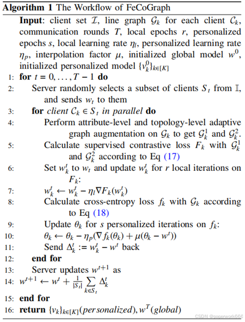
The detailed workflow of FeCoGraph in the personalized FL setting is shown in Algorithm 1. According to the above equations, each client contributes to the shared global model while training a personalized model locally. To accomplish this, we employ the supervised contrastive loss function as the global objective to encourage sharing more fundamental network behavior patterns among clients. Simultaneously, we leverage a supervised cross-entropy loss to capture specific knowledge of the local data distribution. The two objectives are formulated as follows respectively:

个性化联邦学习（FL）设置下FeCoGraph的详细工作流程如算法1所示。根据上述公式，每个客户端在本地训练个性化模型的同时，也为共享的全局模型做出贡献。为此，我们采用有监督的对比损失函数作为全局目标，以鼓励客户端之间共享更多基本的网络行为模式。同时，我们利用有监督的交叉熵损失来捕捉本地数据分布的特定知识。这两个目标分别表述如下：

$$F\left(W_k;{\mathcal{G}}_k\right)$$

$$={\lambda }_{ce}\cdot {\mathcal{L}}_{ce}\left(W_k;{\mathcal{G}}_k\right)+\left(1-{\lambda }_{ce}\right)\cdot {\mathcal{L}}_{\text{supcon }}\left(W_k;{\mathcal{G}}_k\right),\text{\hspace{1em}(17)}$$

$$f\left({\theta }_k;G_k\right)$$

$$={\mathcal{L}}_{ce}\left({\theta }_k;{\mathcal{G}}_k\right)\text{.}\text{\hspace{1em}(18)}$$

V. EXPERIMENTS

五、实验

In this section, we conduct extensive experiments to evaluate the proposed network intrusion detection methods on real-world NIDS datasets. First, we present the necessary information on the experimental setup. Secondly, we report the experiment results attached with performance analysis.

在本节中，我们进行了广泛的实验，以在真实世界的网络入侵检测系统（NIDS）数据集上评估所提出的网络入侵检测方法。首先，我们介绍实验设置的必要信息。其次，我们报告实验结果并附上性能分析。

A. Experimental Setup

A. 实验设置

1. Datasets: We adopt three widely used benchmark datasets to evaluate our method, including NF-BoT-IoT-v2, NF-ToN-IoT-v2, and NF-CSE-CIC-IDS2018-v2 [51]. All of these datasets are netflow datasets. Each data sample is a network traffic flow representing a series of packets between two edge devices. There are total 43 features that show information on general flow statistics and some specific protocols. All flow-based features are extracted from packet headers rather than payload information. The detailed descriptions of each dataset are as follows. The v2 version is an extended version of the corresponding v1 dataset, which contains more samples and statistical features. The detailed statistics of three datasets are shown in Table II

2. 数据集：我们采用三个广泛使用的基准数据集来评估我们的方法，包括NF - BoT - IoT - v2、NF - ToN - IoT - v2和NF - CSE - CIC - IDS2018 - v2 [51]。所有这些数据集都是网络流数据集。每个数据样本是一个网络流量流，代表两个边缘设备之间的一系列数据包。总共有43个特征，显示了一般流量统计信息和一些特定协议的信息。所有基于流的特征都是从数据包头部提取的，而不是从有效负载信息中提取的。每个数据集的详细描述如下。v2版本是相应v1数据集的扩展版本，包含更多的样本和统计特征。三个数据集的详细统计信息如表二所示

• NF-BoT-IoT-v2 is a netflow-based IoT dataset from a network environment in 2018. It contains 37,763,497 flows out of which 37,628,460(99.64%) are malicious and 135,037(0.36%) are benign.

• NF - BoT - IoT - v2是一个基于网络流的物联网数据集，来自2018年的一个网络环境。它包含37,763,497个流量，其中37,628,460（99.64%）个是恶意流量，135,037（0.36%）个是良性流量。

• NF-ToN-IoT-v2 is a netflow-based IoT dataset realized in 2019. It contains 16,940,496 data flows out of which $10,841,027\left(63.99\%\right)$ are malicious and 6,099,469(36.01%) are benign.

• NF - ToN - IoT - v2是一个在2019年实现的基于网络流的物联网数据集。它包含16,940,496个数据流，其中 $10,841,027\left(63.99\%\right)$ 个是恶意的，6,099,469（36.01%）个是良性的。

• NF-CSE-CIC-IDS2018-v2 is a dataset collected in 2018. It contains 18,893,708 network flows, out of which $2,258,141\left(11.95\%\right)$ are malicious and $16,635,567\left(88.05\%\right)$ are benign.

• NF - CSE - CIC - IDS2018 - v2是一个在2018年收集的数据集。它包含18,893,708个网络流量，其中 $2,258,141\left(11.95\%\right)$ 个是恶意的，$16,635,567\left(88.05\%\right)$ 个是良性的。

2. Data Preparation: We perform four pre-processing steps before converting network flows into network graphs. For each flow data, we merge the IP address and port number into one attribute by concatenating two attributes. Since Certain types of attacks are associated with specific port numbers, only IP addresses are not sufficient to distinguish them. The merged attribute are expected to more precisely capture the behavioral patterns associated with different attacks. Secondly, we fill the missing and infinite values with zero. Thirdly, we perform target encoding to convert categorical features into numerical values. The labels indicating benign/malicious and attack type are also transformed into numerical values. Finally, a standard scaler is adopted to obtain the normalized features.

3. 数据准备：在将网络流量转换为网络图之前，我们执行四个预处理步骤。对于每个流量数据，我们通过连接IP地址和端口号这两个属性，将它们合并为一个属性。由于某些类型的攻击与特定的端口号相关，仅使用IP地址不足以区分它们。合并后的属性有望更精确地捕捉与不同攻击相关的行为模式。其次，我们用零填充缺失值和无穷值。第三，我们执行目标编码，将分类特征转换为数值。表示良性/恶意和攻击类型的标签也转换为数值。最后，采用标准缩放器来获得归一化的特征。

TABLE II

ATTACK CATEGORY STATISTICS OF THREE NIDS DATASETS

三个NIDS数据集的攻击类别统计

Dataset	Class Distribution (%)										Total Size
NF-BoT-IoT-v2	Benign 0.36	DDoS 48.54	DoS 44.15	Reconnaissance 6.94	Theft 0.0064						37,763,497
NF-ToN-IoT-v2	Benign	Backdoor	DDoS	DoS	Injection	MITM	Password	Ransomware	Scanning	XSS	16,940,496
	36.01	0.099	11.96	4.21	4.04	0.046	6.81	0.020	22.32	14.49
NF-CSE-CIC-IDS2018-v2	Benign	BruteForce	Bot	DoS	DDoS	Infiltration	Web Attack				18,893,708
	88.05	0.64	0.76	2.56	7.36	0.62	0.019

数据集	类别分布（%）										总大小
NF - 物联网僵尸网络数据集v2（NF - BoT - IoT - v2）	良性 0.36	分布式拒绝服务攻击（DDoS） 48.54	拒绝服务攻击（DoS） 44.15	侦察攻击 6.94	盗窃攻击 0.0064						37,763,497
NF - 物联网流量数据集v2（NF - ToN - IoT - v2）	良性	后门攻击	分布式拒绝服务攻击（DDoS）	拒绝服务攻击（DoS）	注入攻击	中间人攻击（MITM）	密码攻击	勒索软件攻击	扫描攻击	跨站脚本攻击（XSS）	16,940,496
	36.01	0.099	11.96	4.21	4.04	0.046	6.81	0.020	22.32	14.49
NF - 加拿大网络安全实验中心入侵检测数据集2018 v2（NF - CSE - CIC - IDS2018 - v2）	良性	暴力破解攻击	僵尸网络攻击	拒绝服务攻击（DoS）	分布式拒绝服务攻击（DDoS）	渗透攻击	网络攻击				18,893,708
	88.05	0.64	0.76	2.56	7.36	0.62	0.019

3. Baselines: To provide a comprehensive evaluation, We compare our methods with two types of baselines, including machine learning methods and GNN methods.

4. 基线方法：为了进行全面评估，我们将我们的方法与两种类型的基线方法进行比较，包括机器学习方法和图神经网络（GNN）方法。

• The machine learning baseline algorithms include AdaBoost, k Nearest Neighbors (KNN), Decision Tree, and tree-based ensemble methods (XGBoost, Random Forest, Extra Trees). We directly feed network flow-based features into the machine learning classifier.

• 机器学习基线算法包括自适应提升（AdaBoost）、k近邻算法（KNN）、决策树以及基于树的集成方法（XGBoost、随机森林、极端随机树）。我们直接将基于网络流的特征输入到机器学习分类器中。

• We primarily compare our methods with E-graphSAGE [7] to showcase the improvement brought by contrastive learning under few-shot scenarios. It is a supervised approach that adjusts the message propagation mechanism by aggregating edge features instead of node features.

• 我们主要将我们的方法与E-graphSAGE [7]进行比较，以展示少样本场景下对比学习所带来的改进。它是一种有监督的方法，通过聚合边特征而非节点特征来调整消息传播机制。

• Anomal-E [11] is included to demonstrate the effect of label information in contrastive learning. It is built upon an E-graphSAGE encoder, incorporates a modified DGI (Deep Graph Infomax) objective, and integrates four traditional anomaly detection algorithms.

• 纳入Anomal-E [11]是为了展示对比学习中标签信息的作用。它基于E-graphSAGE编码器构建，结合了改进的深度图信息最大化（DGI）目标，并集成了四种传统的异常检测算法。

• we additionally compare our methods with E-ResGAT [8]. It incorporates residual learning into the original GAT architecture to improve the performance of minority classes and stabilize model training.

• 我们还将我们的方法与E-ResGAT [8]进行比较。它将残差学习融入到原始的图注意力网络（GAT）架构中，以提高少数类别的性能并稳定模型训练。

4. Evaluation Metrics: Four metrics are leveraged to evaluate the performance of FeCoGraph, including accuracy, precision, recall, and f1-score. These metrics have been extensively used in numerous previous works. These metrics are calculated with the number of true positive(TP),false positive (FP),true negative(TN)and false negative(FN),which can be formulated as follows:

5. 评估指标：使用四个指标来评估FeCoGraph的性能，包括准确率、精确率、召回率和F1分数。这些指标在许多先前的工作中被广泛使用。这些指标是根据真阳性（TP）、假阳性（FP）、真阴性（TN）和假阴性（FN）的数量计算的，具体公式如下：

$$\text{ Accuracy }=\frac{TP+TN}{TP+FP+TN+FN},\text{\hspace{1em}(19)}$$

the accuracy is calculated as the ratio of correctly predicted samples to all samples in the dataset;

准确率计算为数据集中正确预测的样本数与所有样本数的比率；

$$\text{ Precision }=\frac{TP}{TP+FP},\text{\hspace{1em}(20)}$$

Precision is defined as the ratio of all correctly predicted positive samples to all samples predicted as positive.;

精确率定义为所有正确预测的正样本数与所有预测为正的样本数的比率；

$$\text{ Recall }=\frac{TP}{TP+FN},\text{\hspace{1em}(21)}$$

Recall is defined as the ratio of all correctly predicted positive samples to all actual positive samples in the dataset;

召回率定义为所有正确预测的正样本数与数据集中所有实际正样本数的比率；

$$\mathrm{F}1-\text{ Score }=\frac{2\times \text{ Precision }\times \text{ Recall }}{\text{ Precision }+\text{ Recall }},\text{\hspace{1em}(22)}$$

The F1-score is defined as the harmonic mean of precision and recall. It achieves a balance between two metrics in imbalanced datasets. Note that we use a macro version of the above metrics, which are calculated and equally averaged for each class. Since class distributions are generally imbalanced in network intrusion detection, macro values are appropriate for treating each class equally.

F1分数定义为精确率和召回率的调和平均值。它在不平衡数据集中实现了两个指标之间的平衡。请注意，我们使用上述指标的宏版本，即对每个类别进行计算并取平均。由于网络入侵检测中的类别分布通常是不平衡的，宏值适合平等对待每个类别。

5. Experimental Settings: The proposed algorithm is implemented with PyTorch, DGL and PyTorch Geometric. The backbone encoder is composed of a two-layer graph convolutional network (GCN). The input feature dimension is 39 , which corresponds to the number of network flow features. The number of hidden units in the two layers is set to 64 and 32 respectively. The dimension of projector hidden layers in tuned from the parameter set { 64 , 128 , 256 } \{ {64},{128},{256}\} {64,128,256} ,in which 256 is selected as the optimal value based on validation performance. Datasets were uniformly downsampled by label proportion due to the heavy computation burden of using full dataset, with a downsampling ratio of $2\%$ . Since the volume of network flows is relatively large, we calculate supervised contrastive loss in batches to avoid the issue of CUDA out of memory. All experiments were performed on Ubuntu 22.04 OS equipped with 2 NVIDIA GeForce RTX 3090 GPUs. Relevant software libraries include Python 3.8.8, PyTorch 1.13.0, DGL 1.2, and PyTorch Geometric 2.3.0, etc.

6. 实验设置：所提出的算法使用PyTorch、DGL和PyTorch Geometric实现。骨干编码器由两层图卷积网络（GCN）组成。输入特征维度为39，对应于网络流特征的数量。两层中的隐藏单元数量分别设置为64和32。投影器隐藏层的维度从参数集 { 64 , 128 , 256 } \{ {64},{128},{256}\} {64,128,256}中调整，其中根据验证性能选择256作为最优值。由于使用完整数据集的计算负担较重，数据集按标签比例进行统一降采样，降采样率为$2\%$。由于网络流的数量相对较大，我们分批计算有监督的对比损失，以避免CUDA内存不足的问题。所有实验均在配备2块NVIDIA GeForce RTX 3090 GPU的Ubuntu 22.04操作系统上进行。相关软件库包括Python 3.8.8、PyTorch 1.13.0、DGL 1.2和PyTorch Geometric 2.3.0等。

For machine learning approaches, we directly utilize algorithms to fit training samples and provide prediction results for test samples. For GNN-based approaches, batch gradient descent is leveraged with an Adam optimizer. The models are uniformly trained in 2000 epochs with a learning rate of 0.001 . Following the setting in E-graphSAGE with additional simulation for few-shot NIDS, we split the overall dataset into train and test graphs. $30\%$ of the data is used for training,and the remaining $70\%$ for test. Note that the anomaly detector of Anomal-E is finetuned in an unsupervised manner, it is unfair to compare it with our method. In line with TS-IDS, we exclusively utilize the E-graphSAGE encoder from Anomal-E to produce edge embeddings. These embeddings are then utilized to fine-tune an XGBoost classifier.

对于机器学习方法，我们直接使用算法来拟合训练样本并为测试样本提供预测结果。对于基于GNN的方法，使用Adam优化器进行批量梯度下降。模型统一训练2000个轮次，学习率为0.001。遵循E-graphSAGE中的设置并对少样本网络入侵检测系统（NIDS）进行额外模拟，我们将整个数据集划分为训练图和测试图。$30\%$的数据用于训练，其余$70\%$用于测试。请注意，Anomal-E的异常检测器是以无监督的方式进行微调的，将其与我们的方法进行比较是不公平的。与TS-IDS一致，我们仅使用Anomal-E中的E-graphSAGE编码器来生成边嵌入。然后使用这些嵌入来微调一个XGBoost分类器。

For FL experiments, it is a common practice in FL experiments to split a centralized dataset into multiple partitions and distribute them across different clients. The whole network traffic graph is partitioned into 10 subgraphs based on the Latent Dirichlet Allocation (LDA) Strategy [52]. Specifically, we partition nodes in each class $k$ into $J$ shards following a symmetric Dirichlet distribution ${\mathbf{p}}_k\sim {\mathrm{Dir}}_J\left(\alpha \right)$ ,where client $j$ will be assigned with a shard of ${\mathbf{p}}_{k,j}$ proportion. The total nodes of client $j$ are obtained by gathering each corresponding ${\mathbf{p}}_{k,j}$ partition of class $k$ . Then subgraphs are generated by recovering the original links between some of nodes. For the consideration of few-shot detection, we subsequently keep $30\%$ of the entire nodes labeled. We uniformly set the number of communication rounds and local epochs as 100 and 5 , respectively. Evaluation metrics of each individual client are averaged in FL scenarios. We use best mean testing accuracy (BMTA) [53] as the primary evaluation metric.

在联邦学习（FL）实验中，常见的做法是将集中式数据集分割成多个分区，并将它们分配给不同的客户端。基于潜在狄利克雷分配（Latent Dirichlet Allocation，LDA）策略 [52]，将整个网络流量图划分为 10 个子图。具体来说，我们按照对称狄利克雷分布 ${\mathbf{p}}_k\sim {\mathrm{Dir}}_J\left(\alpha \right)$ 将每个类别 $k$ 中的节点划分为 $J$ 个分片，其中客户端 $j$ 将被分配比例为 ${\mathbf{p}}_{k,j}$ 的一个分片。客户端 $j$ 的总节点数是通过收集类别 $k$ 中每个相应的 ${\mathbf{p}}_{k,j}$ 分区得到的。然后，通过恢复一些节点之间的原始链接来生成子图。考虑到小样本检测，我们随后保留整个节点中 $30\%$ 的节点进行标注。我们将通信轮数和本地训练轮数分别统一设置为 100 和 5。在联邦学习场景中，对每个客户端的评估指标进行平均。我们使用最佳平均测试准确率（Best Mean Testing Accuracy，BMTA） [53] 作为主要评估指标。

TABLE III

Binary and Multiclass Performance Comparison With the State-of-the-art Algorithms. (NF-BoT-IOT-v2 Is Abbreviated as BoT, NF-TON-IOT-V2 Is Abbreviated as TON, NF-CSE-CIC-IDS2018-v2 Is Abbreviated as IDS2018)

与最先进算法的二分类和多分类性能比较。（NF - BoT - IOT - v2 简称为 BoT，NF - TON - IOT - V2 简称为 TON，NF - CSE - CIC - IDS2018 - v2 简称为 IDS2018）

$\mathbf{{Dataset}}$	Binary Classification					Multiclass Classification
	Method	Accuracy	Precision	Recall	F1-Score	Method	Accuracy	Precision	Recall	F1-Score
BoT	KNN	99.64	49.82	50.00	49.91	KNN	46.26	19.97	19.85	19.11
	AdaBoost	99.88	95.95	86.30	90.56	AdaBoost	97.87	60.37	59.31	59.64
	Decision Tree	99.82	95.53	77.36	84.17	Decision Tree	97.84	74.18	73.14	73.65
	XGBoost	99.89	97.84	85.78	90.94	XGBoost	98.46	76.88	75.23	76.01
	E-graphSAGE [7]	99.65	99.82	51.05	51.97	E-graphSAGE [7]	96.81	71.28	72.37	71.81
	Anomal-E [11]	99.87	97.37	83.94	89.54	Anomal-E [11]	96.79	76.07	71.95	73.74
	E-ResGAT [8]	99.74	66.58	40.12	44.57	E-ResGAT [8]	97.95	77.70	64.63	68.26
	$\mathbf{{Ours}}$	99.89	96.92	86.61	91.12	Ours	98.48	98.03	79.92	86.86
ToN	KNN	93.08	93.14	91.76	92.38	KNN	85.35	55.14	51.73	52.7
	AdaBoost	86.64	85.93	88.85	86.24	AdaBoost	44.84	14.23	23.57	15.3
	Decision Tree	96.63	96.56	96.10	96.32	Decision Tree	89.92	70.09	63.66	63.79
	XGBoost	95.60	96.26	94.25	95.12	XGBoost	90.77	73.86	64.52	65.94
	E-graphSAGE [7]	78.47	79.8	82.15	78.25	E-graphSAGE [7]	83.05	69.74	76.88	71.39
	Anomal-E [11]	95.77	95.88	94.89	95.36	Anomal-E [11]	87.26	68.06	61.90	62.12
	E-ResGAT [8]	93.84	94.23	92.46	93.23	E-ResGAT [8]	84.40	63.17	56.68	58.36
	Ours	96.90	96.81	96.44	96.62	Ours	94.32	74.28	72.46	73.31
IDS2018	KNN	87.15	50.36	50.04	47.71	KNN	87.83	13.09	14.26	13.39
	AdaBoost	99.26	98.9	97.56	98.22	AdaBoost	95.3	38.17	41.88	39.71
	Decision Tree	99.07	97.85	97.72	97.79	Decision Tree	98.87	73.65	73.36	72.96
	XGBoost	99.24	98.9	97.74	98.31	XGBoost	99.3	83.83	73.41	74.75
	E-graphSAGE [7]	93.20	92.49	73.40	79.36	E-graphSAGE [7]	92.16	67.44	62.72	61.26
	Anomal-E [11]	91.57	83.03	72.22	76.17	Anomal-E [11]	96.79	76.07	71.95	73.74
	E-ResGAT [8]	98.45	97.34	95.30	96.29	E-ResGAT [8]	98.36	80.62	67.80	68.38
	Ours	99.63	99.38	98.85	99.11	Ours	99.52	84.41	79.07	81.38

$\mathbf{{Dataset}}$	二元分类					多类分类
	方法	准确率	精确率	召回率	F1分数	方法	准确率	精确率	召回率	F1分数
BoT（原文未明确含义，保留英文）	k近邻算法（K-Nearest Neighbors，KNN）	99.64	49.82	50.00	49.91	k近邻算法（K-Nearest Neighbors，KNN）	46.26	19.97	19.85	19.11
	自适应提升算法（AdaBoost）	99.88	95.95	86.30	90.56	自适应提升算法（AdaBoost）	97.87	60.37	59.31	59.64
	决策树	99.82	95.53	77.36	84.17	决策树	97.84	74.18	73.14	73.65
	极端梯度提升算法（XGBoost）	99.89	97.84	85.78	90.94	极端梯度提升算法（XGBoost）	98.46	76.88	75.23	76.01
	E图采样与聚合算法（E-graphSAGE [7]）	99.65	99.82	51.05	51.97	E图采样与聚合算法（E-graphSAGE [7]）	96.81	71.28	72.37	71.81
	Anomal-E [11]（原文未明确含义，保留英文）	99.87	97.37	83.94	89.54	Anomal-E [11]（原文未明确含义，保留英文）	96.79	76.07	71.95	73.74
	E残差图注意力网络（E-ResGAT [8]）	99.74	66.58	40.12	44.57	E残差图注意力网络（E-ResGAT [8]）	97.95	77.70	64.63	68.26
	$\mathbf{{Ours}}$	99.89	96.92	86.61	91.12	我们的方法	98.48	98.03	79.92	86.86
ToN（原文未明确含义，保留英文）	k近邻算法（K-Nearest Neighbors，KNN）	93.08	93.14	91.76	92.38	k近邻算法（K-Nearest Neighbors，KNN）	85.35	55.14	51.73	52.7
	自适应提升算法（AdaBoost）	86.64	85.93	88.85	86.24	自适应提升算法（AdaBoost）	44.84	14.23	23.57	15.3
	决策树	96.63	96.56	96.10	96.32	决策树	89.92	70.09	63.66	63.79
	极端梯度提升算法（XGBoost）	95.60	96.26	94.25	95.12	极端梯度提升算法（XGBoost）	90.77	73.86	64.52	65.94
	E图采样与聚合算法（E-graphSAGE [7]）	78.47	79.8	82.15	78.25	E图采样与聚合算法（E-graphSAGE [7]）	83.05	69.74	76.88	71.39
	Anomal-E [11]（原文未明确含义，保留英文）	95.77	95.88	94.89	95.36	Anomal-E [11]（原文未明确含义，保留英文）	87.26	68.06	61.90	62.12
	E残差图注意力网络（E-ResGAT [8]）	93.84	94.23	92.46	93.23	E残差图注意力网络（E-ResGAT [8]）	84.40	63.17	56.68	58.36
	我们的方法	96.90	96.81	96.44	96.62	我们的方法	94.32	74.28	72.46	73.31
2018年入侵检测数据集（IDS2018）	k近邻算法（K-Nearest Neighbors，KNN）	87.15	50.36	50.04	47.71	k近邻算法（K-Nearest Neighbors，KNN）	87.83	13.09	14.26	13.39
	自适应提升算法（AdaBoost）	99.26	98.9	97.56	98.22	自适应提升算法（AdaBoost）	95.3	38.17	41.88	39.71
	决策树	99.07	97.85	97.72	97.79	决策树	98.87	73.65	73.36	72.96
	极端梯度提升算法（XGBoost）	99.24	98.9	97.74	98.31	极端梯度提升算法（XGBoost）	99.3	83.83	73.41	74.75
	E图采样与聚合算法（E-graphSAGE [7]）	93.20	92.49	73.40	79.36	E图采样与聚合算法（E-graphSAGE [7]）	92.16	67.44	62.72	61.26
	Anomal-E [11]（原文未明确含义，保留英文）	91.57	83.03	72.22	76.17	Anomal-E [11]（原文未明确含义，保留英文）	96.79	76.07	71.95	73.74
	E残差图注意力网络（E-ResGAT [8]）	98.45	97.34	95.30	96.29	E残差图注意力网络（E-ResGAT [8]）	98.36	80.62	67.80	68.38
	我们的方法	99.63	99.38	98.85	99.11	我们的方法	99.52	84.41	79.07	81.38

B. Result Analysis

B. 结果分析

In this part, we first provide binary classification results to validate the ability of FeCoGraph to differentiate benign flows from malicious flows. Secondly, the multiclass classification results are presented to demonstrate FeCoGraph’s capability to identify different attack types. We also investigate the impact of label proportion, supervised contrastive loss, and key hyperparameters. Finally, we illustrate the convergence performance of FeCoGraph under the non-IID data scenario.

在这部分，我们首先给出二分类结果，以验证FeCoGraph区分良性流量和恶意流量的能力。其次，展示多分类结果，以证明FeCoGraph识别不同攻击类型的能力。我们还研究了标签比例、监督对比损失和关键超参数的影响。最后，我们说明FeCoGraph在非独立同分布（non-IID）数据场景下的收敛性能。

1. Binary Classification Performance: To evaluate the ability of our method to discriminate malicious flows from benign flows, we conduct the binary classification experiment under the $30\%$ proportion of labeled samples. The results compared with other representative GNN-based methods are reported in Table III, including accuracy, precision, recall and F1- score. As shown in the table, our solution performs well on three datasets. On the NF-CSE-CIC-IDS2018-v2 dataset, our method achieves the best F1 score and accuracy. On NF-ToN-IoT-v2 dataset, our method obtains an accuracy of 96.9% and an F1-score of 96.62%. On NF-BoT-IoT dataset, our method obtains an accuracy of 99.89% and 91.12% of F1-score, achieving the pinnacle of performance on these two datasets. Furthermore, our method exhibits commendable results when compared with graph-based methods, which demonstrate the potential utility of supervised contrastive loss to learn compact intra-class representations. Finally, tree-based ensemble learning methods obtain competitive results on all datasets, which indicates that ensemble learning has led to significant performance improvement than individual classifiers alone.

2. 二分类性能：为了评估我们的方法区分恶意流量和良性流量的能力，我们在标记样本比例为$30\%$的情况下进行了二分类实验。与其他有代表性的基于图神经网络（GNN）的方法的比较结果报告在表III中，包括准确率、精确率、召回率和F1分数。如表所示，我们的解决方案在三个数据集上表现良好。在NF - CSE - CIC - IDS2018 - v2数据集上，我们的方法取得了最佳的F1分数和准确率。在NF - ToN - IoT - v2数据集上，我们的方法获得了96.9%的准确率和96.62%的F1分数。在NF - BoT - IoT数据集上，我们的方法获得了99.89%的准确率和91.12%的F1分数，在这两个数据集上达到了性能的顶峰。此外，与基于图的方法相比，我们的方法表现出了值得称赞的结果，这证明了监督对比损失在学习紧凑的类内表示方面的潜在效用。最后，基于树的集成学习方法在所有数据集上都取得了有竞争力的结果，这表明集成学习比单个分类器单独使用能显著提高性能。

2) Multiclass Classification Performance:

2) 多分类性能：

a) Comparison with State-of-the-Art Algorithms: To evaluate the ability to accurately discriminate various attack categories, the multiclass classification experiment is conducted with $30\%$ proportions of labeled samples,the same setting as in binary classification. On NF-CSE-CIC-IDS- 2018v2 dataset, our method achieves the best accuracy of 99.52% and the best F1-score of 81.38%. Moreover, the F1-score achieved by our methods is substantially ahead of other methods, surpassing XGBoost and obtaining second-best results by $6.61\%$ . Results on both datasets suggest our method has advanced capabilities to detect genuine threats while minimizing the risk of false alarms. Similarly, On NF-BoT-IoT-v2 dataset, our method outperforms other methods across four metrics. On NF-ToN-IoT-v2 dataset, our method achieves the best detection performance, with an accuracy of $94.32\%$ and a F1-score of 73.31%.

a) 与最先进算法的比较：为了评估准确区分各种攻击类别的能力，在标记样本比例为$30\%$的情况下进行了多分类实验，设置与二分类相同。在NF - CSE - CIC - IDS - 2018v2数据集上，我们的方法取得了99.52%的最佳准确率和81.38%的最佳F1分数。此外，我们的方法获得的F1分数大幅领先于其他方法，超过了XGBoost（极端梯度提升），并以$6.61\%$的优势获得了第二好的结果。两个数据集上的结果表明，我们的方法具有先进的能力来检测真正的威胁，同时将误报风险降至最低。同样，在NF - BoT - IoT - v2数据集上，我们的方法在四个指标上都优于其他方法。在NF - ToN - IoT - v2数据集上，我们的方法实现了最佳的检测性能，准确率为$94.32\%$，F1分数为73.31%。

An interesting phenomenon is that tree-based ensemble learning methods have showcased a universally high performance on NF-ToN-IoT-v2 dataset for both binary and multiclass classification, in contrast to the performance on NF-CSE-CIC-IDS2018-v2 dataset. It can be inferred that these methods are sufficient to capture complex patterns and relationships within the data. Besides, the gap between the performance of our method and the best performance achieved by the Random Forest algorithm is smaller than that in a binary classification task, showing the superiority of our methods in distinguishing different network flows via line graph construction.

一个有趣的现象是，基于树的集成学习方法在NF - ToN - IoT - v2数据集的二分类和多分类任务中都表现出普遍较高的性能，这与它们在NF - CSE - CIC - IDS2018 - v2数据集上的表现形成对比。可以推断，这些方法足以捕捉数据中的复杂模式和关系。此外，我们的方法的性能与随机森林算法取得的最佳性能之间的差距比二分类任务中的差距更小，这显示了我们的方法通过线图构建在区分不同网络流量方面的优越性。

Fig. 3. F1-score for each attack scenario on NF-BoT-IoT-v2 dataset.

图3. NF - BoT - IoT - v2数据集上每个攻击场景的F1分数。

Fig. 4. F1-score for each attack scenario on NF-ToN-IoT-v2 dataset.

图4. NF - ToN - IoT - v2数据集上每个攻击场景的F1分数。

b) Detection Performance on Attack Categories: With the presence of numerous emerging and complicated cyber attacks, it’s critical to differentiate between malicious flows and benign flows and further distinguish different types of abnormal behaviors. Moreover, different types of malicious flows exhibit a skewed distribution, where certain types of attacks occur more frequently than others. We compare our method with E-graphSAGE, one of the state-of-the-art GNN-based approaches, in terms of F1-score values for each category on NF-BoT-IoT-V2, NF-ToN-IoT-v2 and NF-CSE-CIC-IDS2018-v2. The proportion of labeled samples is set to $30\%$ on both datasets.

b) 对攻击类别的检测性能：随着众多新兴和复杂的网络攻击的出现，区分恶意流量和良性流量并进一步区分不同类型的异常行为至关重要。此外，不同类型的恶意流量呈现出偏态分布，某些类型的攻击比其他类型更频繁发生。我们在NF - BoT - IoT - V2、NF - ToN - IoT - v2和NF - CSE - CIC - IDS2018 - v2数据集上，就每个类别的F1分数值，将我们的方法与最先进的基于GNN的方法之一E - graphSAGE进行了比较。两个数据集上的标记样本比例都设置为$30\%$。

Figure 3 provides the results on NF-BoT-IoT-v2. It includes 4 attack scenarios: Reconnaissance, DDoS, DoS, and Theft. As shown in the Table, our approach consistently outperforms E-graphSAGE for all attack scenarios. Especially, E-graphSAGE cannot effectively identify Theft attacks due to scarce samples, while our approach achieves an F1-score of $57.14\%$ . Theft aims to obtain sensitive data via some disguised ways, such as social engineering. The results demonstrate the ability of our approach to detect rare and covert attacks

图3给出了在NF - BoT - IoT - v2上的结果。它包括4种攻击场景：侦察、分布式拒绝服务（DDoS）、拒绝服务（DoS）和盗窃。如表所示，在所有攻击场景中，我们的方法始终优于E - graphSAGE。特别是，由于样本稀缺，E - graphSAGE无法有效识别盗窃攻击，而我们的方法实现了$57.14\%$的F1分数。盗窃攻击旨在通过一些伪装手段（如社会工程学）获取敏感数据。结果证明了我们的方法检测罕见和隐蔽攻击的能力。

Figure 4 provides the results on NF-ToN-IoT-v2. It includes 9 attack scenarios: backdoor, DoS, DDoS, injection, MITM, password, ransomware, scanning and XSS. As seen in the table, the F1-score of E-graphsage for injection, DDoS and XSS is $48.36\%,59.37\%$ and $73.56\%$ ,respectively. On the one hand, the number of samples for these three scenarios is relatively small, so it’s difficult for the model to capture the behavior patterns of these categories of attacks. On the other hand, these attacks are more easily misclassified as normal network flows. Injection involves manipulating or injecting malicious code into data streams to alter the execution path, Cross-site Scripting (XSS) is also a type of injection operated in web applications. DDoS is a distributed DoS attack launched by many hosts, attackers can lower the attack rate of DoS to evade detection. Compared with E-graphSAGE, our method introduces a supervised contrastive objective along with a refined graph convolution process via line graph construction. After these operations, the F1-score against DDoS attacks has improved from 59.37% to 87.96%. The F1-score against Injection attack has improved from 48.36% to 76.36%. The F1 score against XSS attack has increased from 73.56% to 92.57%. Note that E-graphSAGE performs better than our methods against Man-In-The-Middle (MITM) and ransomware attacks, which are two extremely rare attack scenarios.

图4展示了在NF - ToN - IoT - v2上的实验结果。它包含9种攻击场景：后门攻击、拒绝服务攻击（DoS）、分布式拒绝服务攻击（DDoS）、注入攻击、中间人攻击（MITM）、密码攻击、勒索软件攻击、扫描攻击和跨站脚本攻击（XSS）。从表中可以看出，E - graphsage在注入攻击、DDoS攻击和XSS攻击上的F1分数分别为$48.36\%,59.37\%$和$73.56\%$。一方面，这三种场景的样本数量相对较少，因此模型难以捕捉这些类别攻击的行为模式。另一方面，这些攻击更容易被误分类为正常网络流量。注入攻击涉及将恶意代码操纵或注入到数据流中以改变执行路径，跨站脚本攻击（XSS）也是一种在Web应用程序中进行的注入攻击。DDoS是由许多主机发起的分布式DoS攻击，攻击者可以降低DoS攻击的速率以逃避检测。与E - graphSAGE相比，我们的方法通过线图构建引入了有监督的对比目标以及精细的图卷积过程。经过这些操作后，针对DDoS攻击的F1分数从59.37%提高到了87.96%。针对注入攻击的F1分数从48.36%提高到了76.36%。针对XSS攻击的F1分数从73.56%提高到了92.57%。需要注意的是，在中间人攻击（MITM）和勒索软件攻击这两种极为罕见的攻击场景中，E - graphSAGE的表现优于我们的方法。

Fig. 5. F1-score for each attack scenario on NF-CSE-CIC-IDS2018-v2 dataset.

图5. NF - CSE - CIC - IDS2018 - v2数据集上各攻击场景的F1分数。

Fig. 6. Visualization of reduction (a) raw edge features from NF-CSE-CIC2018-v2 test set. (b) edge embeddings generated by FeCoGraph encoder.

图6. 降维可视化 (a) 来自NF - CSE - CIC2018 - v2测试集的原始边特征。(b) FeCoGraph编码器生成的边嵌入。

The NF-CSE-CIC-IDS2018-v2 dataset covers 6 attack scenarios, including BruteForce, bot, DoS, DDoS, infiltration, and Web Attacks. As seen in Figure 5, the F1-score of E-graphSAGE against DoS and infiltration attack is only $34.04\%$ and $14.59\%$ ,respectively. In addition to the difficulty of detecting DoS mentioned above, infiltration is another type of intricate attack. Infiltration may involve insiders with legitimate access to the system and employ stealth techniques to avoid detection. After employing a supervised contrastive objective, the F1-score against DoS attack has improved from $34.04\%$ to $99.14\%$ . Our method also brings a huge increase to the F1-score against infiltration attack,from 14.59% to $82.76\%$ . The considerable performance improvement on two datasets has demonstrated the effect of supervised contrastive learning on classifying different types of malicious flows.

NF - CSE - CIC - IDS2018 - v2数据集涵盖6种攻击场景，包括暴力破解攻击、僵尸网络攻击、拒绝服务攻击（DoS）、分布式拒绝服务攻击（DDoS）、渗透攻击和Web攻击。如图5所示，E - graphSAGE在DoS攻击和渗透攻击上的F1分数分别仅为$34.04\%$和$14.59\%$。除了上述提到的检测DoS攻击的难度外，渗透攻击是另一种复杂的攻击。渗透攻击可能涉及拥有系统合法访问权限的内部人员，并采用隐身技术来避免被检测到。采用有监督的对比目标后，针对DoS攻击的F1分数从$34.04\%$提高到了$99.14\%$。我们的方法还使针对渗透攻击的F1分数大幅提高，从14.59%提高到了$82.76\%$。在两个数据集上的显著性能提升证明了有监督对比学习在对不同类型恶意流量进行分类方面的效果。

Fig. 7. Performance of FeCoGraph on specific categories with different label proportions. (a) NF-CSE-CIC-IDS2018-v2 dataset; (b) NF-ToN-IoT-v2 dataset.

图7. FeCoGraph在不同标签比例的特定类别上的性能。(a) NF - CSE - CIC - IDS2018 - v2数据集；(b) NF - ToN - IoT - v2数据集。

To intuitively demonstrate the discrimination ability for different attacks, we visualize the raw edge features and edge embeddings generated by the GCN encoder of FeCoGraph. The graph data are sampled from NF-CSE-CIC-IDS2018- v2 dataset. We apply the t-distributed Stochastic Neighbor Embedding (t-SNE) [54] algorithm to map the high-level representation into two dimensions. The result is shown in Fig. 6. In Figure 6a, a large number of malicious flows are mixed with dominant normal flows. Samples of DDoS and DoS attacks cannot be easily differentiated. On the contrary, We can observe clear boundaries between different attacks(e.g., Dos, DDoS) and more compact distribution(e.g., Benign) in Figure 6b. This illustrates the effect of the supervised contrastive objective of separating different traffic flows in the embedding space, which in turn promotes the detection performance.

为了直观地展示对不同攻击的区分能力，我们将FeCoGraph的GCN编码器生成的原始边特征和边嵌入进行可视化。图数据是从NF - CSE - CIC - IDS2018 - v2数据集采样得到的。我们应用t - 分布随机邻域嵌入（t - SNE）[54]算法将高维表示映射到二维空间。结果如图6所示。在图6a中，大量恶意流量与占主导地位的正常流量混合在一起。DDoS攻击和DoS攻击的样本不容易区分。相反，在图6b中，我们可以观察到不同攻击（如DoS、DDoS）之间有清晰的边界，并且分布更加紧凑（如良性流量）。这说明了有监督对比目标在嵌入空间中分离不同流量的效果，进而提升了检测性能。

c) The Impact of Different Label Proportions: To further investigate the performance of our method for varied amounts of training data, we conduct a series of experiments with 10%, $30\%,50\%$ and $70\%$ labeled samples on NF-ToN-IoT-v2 and NF-CSE-CIC-IDS2018-v2 datasets. As seen in Figure 7a, the performances achieved when label proportion is $10\%$ and $30\%$ on NF-CSE-CIC-IDS2018-v2 dataset don’t exhibit a large gap compared to those achieved when utilizing $50\%$ and $70\%$ labeled samples. It can be inferred that our method is capable of learning discriminate flow representations to distinguish different attack categories with critically limited training data.

c) 不同标签比例的影响：为了进一步研究我们的方法在不同数量训练数据下的性能，我们在NF - ToN - IoT - v2和NF - CSE - CIC - IDS2018 - v2数据集上，分别使用10%、$30\%,50\%$和$70\%$的标记样本进行了一系列实验。如图7a所示，在NF - CSE - CIC - IDS2018 - v2数据集上，当标签比例为$10\%$和$30\%$时所取得的性能，与使用$50\%$和$70\%$标记样本时所取得的性能相比，没有出现较大差距。由此可以推断，我们的方法能够在训练数据极为有限的情况下，学习到有区分性的流表示，以区分不同的攻击类别。

TABLE IV

MULTICLASS CLASSIFICATION PERFORMANCE WITH $\lambda$

使用$\lambda$时的多类别分类性能

Dataset	$\lambda$	Accuracy	Precision	Recall	F1-Score
NF-BoT-IoT-v2	0.03	98.48	84.01	95.03	86.94
	0.05	98.46	83.95	94.71	86.73
	0.07	98.47	82.53	94.67	85.25
	0.3	98.43	85.81	94.22	88.31
	0.5	98.46	82.60	94.71	85.30
	0.7	98.47	82.21	94.73	85.13
NF-ToN-IoT-v2	0.03	92.10	72.22	67.67	69.25
	0.05	93.34	73.06	71.07	71.99
	0.07	94.07	74.12	72.23	73.10
	0.3	94.24	74.19	72.40	73.22
	0.5	94.32	74.28	72.46	73.31
	0.7	94.21	74.13	72.35	73.18
NF-CSE-CIC-IDS2018-v2	0.03	98.86	70.14	68.26	69.13
	0.05	99.38	84.43	76.42	79.40
	0.07	99.50	84.39	78.95	81.29
	0.3	99.52	84.03	79.13	81.27
	0.5	99.50	84.15	78.83	81.13
	0.7	99.37	84.41	76.23	79.28

数据集	$\lambda$	准确率	精确率	召回率	F1分数
NF-BoT-IoT-v2	0.03	98.48	84.01	95.03	86.94
	0.05	98.46	83.95	94.71	86.73
	0.07	98.47	82.53	94.67	85.25
	0.3	98.43	85.81	94.22	88.31
	0.5	98.46	82.60	94.71	85.30
	0.7	98.47	82.21	94.73	85.13
NF-ToN-IoT-v2	0.03	92.10	72.22	67.67	69.25
	0.05	93.34	73.06	71.07	71.99
	0.07	94.07	74.12	72.23	73.10
	0.3	94.24	74.19	72.40	73.22
	0.5	94.32	74.28	72.46	73.31
	0.7	94.21	74.13	72.35	73.18
NF-CSE-CIC-IDS2018-v2	0.03	98.86	70.14	68.26	69.13
	0.05	99.38	84.43	76.42	79.40
	0.07	99.50	84.39	78.95	81.29
	0.3	99.52	84.03	79.13	81.27
	0.5	99.50	84.15	78.83	81.13
	0.7	99.37	84.41	76.23	79.28

TABLE V

MULTICLASS CLASSIFICATION PERFORMANCE WITH $\tau$

使用 $\tau$ 的多类别分类性能

Dataset	$\tau$	Accuracy	Precision	Recall	F1-Score
NF-BoT-IoT-v2	0.1	98.48	84.01	95.03	86.94
	0.3	98.46	83.97	94.87	86.83
	0.5	98.46	83.97	94.87	86.83
	0.7	98.47	89.17	95.06	91.44
NF-ToN-IoT-v2	0.1	94.17	73.94	72.33	73.07
	0.3	94.32	74.28	72.46	73.31
	0.5	94.25	74.11	72.41	73.20
	0.7	92.78	73.74	70.12	71.52
NF-CSE-CIC-IDS2018-v2	0.1	99.52	84.03	79.13	81.27
	0.3	99.51	84.30	78.95	81.25
	0.5	99.38	84.44	76.35	79.37
	0.7	99.39	84.45	76.36	79.37

数据集	$\tau$	准确率	精确率	召回率	F1分数
NF-BoT-IoT-v2	0.1	98.48	84.01	95.03	86.94
	0.3	98.46	83.97	94.87	86.83
	0.5	98.46	83.97	94.87	86.83
	0.7	98.47	89.17	95.06	91.44
NF-ToN-IoT-v2	0.1	94.17	73.94	72.33	73.07
	0.3	94.32	74.28	72.46	73.31
	0.5	94.25	74.11	72.41	73.20
	0.7	92.78	73.74	70.12	71.52
NF-CSE-CIC-IDS2018-v2	0.1	99.52	84.03	79.13	81.27
	0.3	99.51	84.30	78.95	81.25
	0.5	99.38	84.44	76.35	79.37
	0.7	99.39	84.45	76.36	79.37

As shown in Figure 7b, There is a little different tendency in detection results on NF-ToN-IoT-v2 dataset, where the f1- score against DDoS, injection, password and XSS attacks increases with the larger proportion of labeled data. It can be observed that these types of attacks are harder to detect, therefore more labeled data is required for our model to enhance the expressive ability of network flow representations for different attack categories. Note that our method always almost fails to detect some particular attack categories, such as web attacks, MITM attack and ransomware attack since there are few samples.

如图7b所示，在NF - ToN - IoT - v2数据集的检测结果中存在一些不同的趋势，其中针对分布式拒绝服务（DDoS）、注入、密码和跨站脚本（XSS）攻击的f1分数随着标记数据比例的增大而提高。可以观察到，这些类型的攻击更难检测，因此我们的模型需要更多的标记数据来增强不同攻击类别网络流量表示的表达能力。请注意，由于样本较少，我们的方法几乎总是无法检测到某些特定的攻击类别，如网络攻击、中间人（MITM）攻击和勒索软件攻击。

d) Detection Performance with Different $\lambda$ and $\tau :\lambda$ and $\tau$ are two important factors in constructing a supervised contrastive loss function. Consequently, we perform a sensitivity analysis to examine how different values affect detection performance. The values of $\lambda$ include0.03,0.05,0.07,0.3, 0.5 and 0.7. The values of $\tau$ include $0.1,0.3,0.5,0.7.\lambda$ weighs the significance of label-aware contrastive loss over supervised learning loss. The smaller $\lambda$ is,the more weight is given to minimize the distances between samples belonging to the same attack category. As shown in Table IV, the four metrics on NF-ToN-IoT-v2 consistently continue to increase and achieve the best results when $\lambda$ is 0.5 . The best F1-score is achieved when $\lambda$ is 0.03 on NF-BoT-IoT-v2 and 0.07 on NF-CSE-CIC-IDS2018-v2, implying that learning class-aware compact representation is more encouraged.

d) 不同$\lambda$和$\tau :\lambda$以及$\tau$下的检测性能 $\lambda$和$\tau :\lambda$以及$\tau$是构建有监督对比损失函数的两个重要因素。因此，我们进行了敏感性分析，以研究不同的值如何影响检测性能。$\lambda$的值包括0.03、0.05、0.07、0.3、0.5和0.7。$\tau$的值包括 $0.1,0.3,0.5,0.7.\lambda$权衡了标签感知对比损失相对于有监督学习损失的重要性。$\lambda$越小，就越会着重最小化属于同一攻击类别的样本之间的距离。如表IV所示，在NF - ToN - IoT - v2上的四个指标持续上升，并在$\lambda$为0.5时达到最佳结果。在NF - BoT - IoT - v2上，当$\lambda$为0.03时达到最佳F1分数；在NF - CSE - CIC - IDS2018 - v2上，当$\lambda$为0.07时达到最佳F1分数，这意味着更鼓励学习类别感知的紧凑表示。

TABLE VI

MULTICLASS CLASSIFICATION RESULTS OF ABLATION STUDY ON CONTRASTIVE LOSS. “SUPCON” DENOTES LABEL-AWARE GRAPH CONTRASTIVE LEARNING MODULE, AND “SSLCON” DENOTES SELF-SUPERVISED GRAPH CONTRASTIVE LEARNING MODULE

对比损失消融研究的多类分类结果。“SUPCON”表示标签感知图对比学习模块，“SSLCON”表示自监督图对比学习模块

Dataset	Task	Setting	Accuracy	Precision	Recall	F1-Score
NF-ToN-IoT-v2	Binary	SupCon	96.90	96.81	96.44	96.62
		SSLcon	92.02	91.01	92.03	91.46
	Multiclass	SupCon	94.32	74.28	72.46	73.31
		SSLCon	91.59	72.41	66.89	68.78
NF-CSE-CIC-IDS2018-v2	Binary	SupCon	99.63	99.38	98.85	99.11
		SSLCon	95.26	87.12	92.34	89.48
	Multiclass	SupCon	99.52	84.41	79.07	81.38
		SSLCon	93.69	23.84	25.43	24.60

数据集	任务	设置	准确率	精确率	召回率	F1分数
NF-ToN-IoT-v2（原文未变，可能是特定数据集名称）	二元的	监督对比学习（SupCon，Supervised Contrastive Learning）	96.90	96.81	96.44	96.62
		SSLcon（原文未变，可能是特定方法或模型名称）	92.02	91.01	92.03	91.46
	多分类	监督对比学习（SupCon，Supervised Contrastive Learning）	94.32	74.28	72.46	73.31
		SSLCon（原文未变，可能是特定方法或模型名称）	91.59	72.41	66.89	68.78
NF-CSE-CIC-IDS2018-v2（原文未变，可能是特定数据集名称）	二元的	监督对比学习（SupCon，Supervised Contrastive Learning）	99.63	99.38	98.85	99.11
		SSLCon（原文未变，可能是特定方法或模型名称）	95.26	87.12	92.34	89.48
	多分类	监督对比学习（SupCon，Supervised Contrastive Learning）	99.52	84.41	79.07	81.38
		SSLCon（原文未变，可能是特定方法或模型名称）	93.69	23.84	25.43	24.60

$\tau$ is associated with the temperature parameter,which affects the sharpness of the probability distribution used in the contrastive loss function. A higher $\tau$ (e.g.,larger temperature) results in a more uniform distribution over similarities, potentially improving generalization. On the other hand, a lower $\tau$ (e.g.,smaller temperature) sharpens the distribution, focusing on maximizing the similarity with positive instances. As shown in Table V,the best results are obtained when $\tau$ is 0.3 on NF-ToN-IoT-v2 and 0.1 on NF-CSE-CIC-IDS2018- v2, showing that supervised contrastive loss tends to impose more penalties on hard negative examples. On the contrary, the best results are obtained when $\tau$ is 0.7 on NF-BoT-IoT-v2, indicating the tendency to encourage global uniformity of flow representation.

$\tau$与温度参数相关，该参数会影响对比损失函数中使用的概率分布的锐度。较高的$\tau$（例如，较大的温度）会使相似度分布更加均匀，有可能提高泛化能力。另一方面，较低的$\tau$（例如，较小的温度）会使分布更加尖锐，专注于最大化与正样本的相似度。如表五所示，在NF - ToN - IoT - v2数据集上，当$\tau$为0.3时取得最佳结果；在NF - CSE - CIC - IDS2018 - v2数据集上，当$\tau$为0.1时取得最佳结果，这表明有监督对比损失倾向于对难负样本施加更多惩罚。相反，在NF - BoT - IoT - v2数据集上，当$\tau$为0.7时取得最佳结果，这表明倾向于鼓励流表示的全局一致性。

e) Ablation Study: Compared with self-supervised contrastive learning that seeks to reduce the distance of multi-view embeddings, label-aware contrastive learning leverages label information to learn compact intra-class representation, we conduct an ablation study to compare the impact of these two objectives in both binary and multiclass classification scenarios. As shown in Table VI, the label-aware contrastive loss function consistently outperforms the counterpart that incorporates self-supervised contrastive learning. On the one hand, the F1-score improves by 5.16% and 4.53% for binary and mul-ticlass classification on NF-ToN-IoT-v2 dataset. On the other hand,the F1-score improves by 9.63% and 56.78% for binary and multiclass classification on NF-CSE-CIC-IDS2018-v2 dataset. The improvements indicate that supervised contrastive learning enables more effective use of unlabeled data, thereby more accurately distinguishing different attacks.

e) 消融实验：与旨在缩小多视图嵌入距离的自监督对比学习相比，标签感知对比学习利用标签信息来学习紧凑的类内表示。我们进行了消融实验，以比较这两个目标在二分类和多分类场景中的影响。如表六所示，标签感知对比损失函数始终优于包含自监督对比学习的对应方法。一方面，在NF - ToN - IoT - v2数据集上，二分类和多分类的F1分数分别提高了5.16%和4.53%。另一方面，在NF - CSE - CIC - IDS2018 - v2数据集上，二分类和多分类的F1分数分别提高了9.63%和56.78%。这些改进表明，有监督对比学习能够更有效地利用未标记数据，从而更准确地区分不同的攻击。

3. The Convergence Performance of FeCoGraph: As discussed before, federated learning is an effective strategy for building distributed intrusion detection systems. To this end, experiments are designed to evaluate the performance of our intrusion detection model in the federated learning scenario. The NetFlow data owned by each client follows non-IID distribution for different attack categories. The traffic data are then converted into a line graph following the paradigm in Section IV-B1. During training, each client trains a local GNN model with a supervised contrastive learning objective. The local parameters are subsequently uploaded into a central server for weight aggregation (e.g., weight-averaging rule).

4. FeCoGraph的收敛性能：如前所述，联邦学习是构建分布式入侵检测系统的有效策略。为此，我们设计了实验来评估我们的入侵检测模型在联邦学习场景中的性能。每个客户端拥有的网络流（NetFlow）数据针对不同的攻击类别遵循非独立同分布（non - IID）。然后，按照第四节B1中的范式将流量数据转换为线图。在训练过程中，每个客户端使用有监督对比学习目标训练一个局部图神经网络（GNN）模型。随后，将局部参数上传到中央服务器进行权重聚合（例如，权重平均规则）。

To ensure a fair evaluation, We compare the performance of three federated learning algorithms. 1) we adopt a vanilla GCN-based FL method to detect malicious flows. 2) we utilize the proposed FeCoGraph intrusion detection model with a supervised contrastive objective in FedAvg. 3) We incorporate the FeCoGraph model with supervised contrastive objective into a personalized FL framework. As shown in Figure, our model with supervised contrastive loss outperforms the counterpart without supervised contrastive loss in terms of detection accuracy, which exhibits similar trends as nonfederated experiments. The green curve shows Personalized FL converges faster and achieves better convergence performance compared with other FL settings, demonstrating the capability of supervised contrasting along with personalization strategy in non-IID federated learning scenarios.

为了确保公平评估，我们比较了三种联邦学习算法的性能。1) 我们采用基于普通图卷积网络（GCN）的联邦学习方法来检测恶意流。2) 我们在联邦平均（FedAvg）算法中使用提出的具有有监督对比目标的FeCoGraph入侵检测模型。3) 我们将具有有监督对比目标的FeCoGraph模型纳入个性化联邦学习框架。如图所示，我们的具有有监督对比损失的模型在检测准确率方面优于没有有监督对比损失的对应模型，这与非联邦实验呈现出相似的趋势。绿色曲线表明，与其他联邦学习设置相比，个性化联邦学习收敛更快，并且实现了更好的收敛性能，这证明了在非独立同分布联邦学习场景中，有监督对比与个性化策略相结合的能力。

Fig. 8. The performance comparison of three FL algorithms.

图8. 三种联邦学习算法的性能比较。

Fig. 9. The performance comparison between FedAvg and personalized FL under shard and dirichlet distribution.

图9. 在分片和狄利克雷分布下，联邦平均（FedAvg）和个性化联邦学习的性能比较。

We further investigate the impact of non-IID factors, including subgraph partition strategy and imbalance level of the Dirichlet distribution. As shown in Figure 9, the personalized FL method (abbreviated as perFL) exhibits a marginal improvement compared with FedAvg. It implies a bi-level optimization strategy can effectively avoid model degradation caused by the issue of client drift. Moreover, the increase in accuracy is more pronounced with the shard partition strategy $\left(12.41\%\text{ vs }3.52\%\right)$ . Since perFL aims to maintain local data distribution, it benefits more when training and test data share a consistent class label distribution. Moreover, Fig 10 demonstrates a decreased tendency of model performance when the Dirichlet distribution tends to be more balanced, where the best result is achieved under the most imbalanced setting. It demonstrates that personalized FL is more compatible with federated NIDS on heterogeneous networks.

我们进一步研究了非独立同分布因素的影响，包括子图划分策略和狄利克雷分布的不平衡程度。如图9所示，个性化联邦学习方法（缩写为perFL）与联邦平均（FedAvg）相比有轻微改进。这意味着双层优化策略可以有效避免由客户端漂移问题导致的模型退化。此外，使用分片划分策略$\left(12.41\%\text{ vs }3.52\%\right)$时，准确率的提升更为明显。由于个性化联邦学习旨在保持局部数据分布，因此当训练数据和测试数据具有一致的类别标签分布时，它会受益更多。此外，图10表明，当狄利克雷分布趋于更加平衡时，模型性能呈下降趋势，在最不平衡的设置下取得最佳结果。这表明个性化联邦学习更适合异构网络上的联邦网络入侵检测系统（NIDS）。

Fig. 10. The performance comparison under different $\alpha$ of the dirichlet distribution.

图10. 在不同狄利克雷分布参数$\alpha$下的性能比较。

VI. CONCLUSION

六、结论

In this paper, we propose FeCoGraph, a label-aware federated graph contrastive learning framework for few-shot intrusion detection. FeCoGraph constructs a label-aware graph contrastive module, promoting the discriminative and expressive capabilities of network flow representations. Furthermore, We incorporate graph contrastive learning module into a personalized FL algorithm to support distributed IDS in edge IoT. Experiment Results on three public datasets show the superiority of FeCoGraph with an average accuracy of 98.27% on binary classification and $96.92\%$ on multiclass classification. In particular, our methods can effectively identify rare and stealthy types of attacks, including DDoS, injection, and infiltration attacks.

在本文中，我们提出了FeCoGraph（标签感知联邦图对比学习框架），这是一种用于少样本入侵检测的标签感知联邦图对比学习框架。FeCoGraph构建了一个标签感知图对比模块，提升了网络流量表示的判别能力和表达能力。此外，我们将图对比学习模块融入到个性化联邦学习（FL）算法中，以支持边缘物联网中的分布式入侵检测系统（IDS）。在三个公共数据集上的实验结果表明，FeCoGraph具有优越性，二分类平均准确率达到98.27%，多分类准确率达到$96.92\%$。特别是，我们的方法能够有效识别罕见和隐蔽的攻击类型，包括分布式拒绝服务（DDoS）攻击、注入攻击和渗透攻击。